
Content#
Exploratory Data Analysis (EDA)
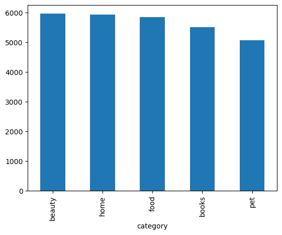
3.1. Product Distribution by Category
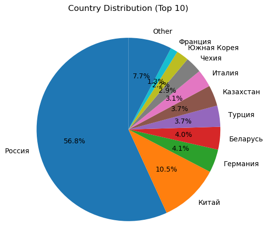
3.2. Product Distribution by Country
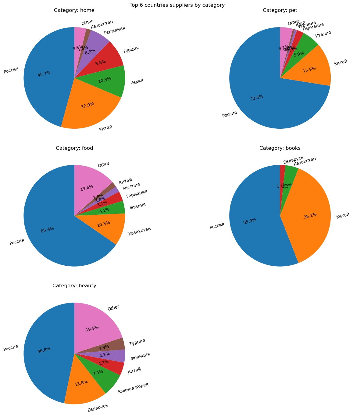
3.3. Product Distribution by Country and Category
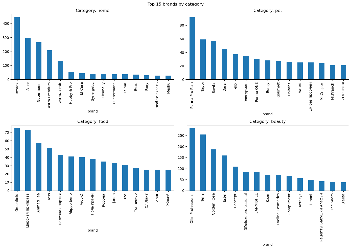
3.4. Product Distribution by Brand and Category
Voice of Customer (VoC) & Root Cause Analysis
6.1. Text Cleaning and Preprocessing
6.2. Tag-to-Review Similarity Matching
6.3. Draft Test Set Construction
6.4. Issue Tag Classification (RCA Taxonomy)
6.4.1 Unsupervised Methods
6.4.2 Semi-Supervised Methods
Read Data#
df_products = pd.read_csv('data/products.csv')
df_products.head()
| id | name | category | rating | price_kzt | author | url | detail_info | ai_positive_tags | ai_negative_tags | ai_summary_text | country | brand | |
|---|---|---|---|---|---|---|---|---|---|---|---|---|---|
| 0 | 2657408 | ПНК «Красная нить» Нить особо прочная, цвет кр... | home | 4.9 | 502.0 | NaN | https://www.flip.kz/catalog?prod=2657408 | {'Бренд': 'ПНК «Красная нить»', 'Страна-произв... | ['прочность', 'тонкая нить', 'подходит для кожи'] | NaN | Мнение клиентов: Нить отмечают за высокую проч... | Россия | ПНК «Красная нить» |
| 1 | 2567952 | Унисон Комплект полотенец вафельных «Let it Snow» | home | 4.8 | 3115.0 | NaN | https://www.flip.kz/catalog?prod=2567952 | {'Торговая марка': 'Унисон', 'Документ о соотв... | ['красивый принт', 'праздничный дизайн', 'боль... | NaN | Мнение клиентов: Покупатели отмечают привлекат... | Россия | NaN |
| 2 | 2657424 | ПНК «Красная нить» Нить особо прочная, цвет ко... | home | 4.9 | 502.0 | NaN | https://www.flip.kz/catalog?prod=2657424 | {'Бренд': 'ПНК «Красная нить»', 'Страна-произв... | ['прочность', 'тонкая нить', 'подходит для кожи'] | NaN | Мнение клиентов: Нить отмечают за высокую проч... | Россия | ПНК «Красная нить» |
| 3 | 1160459 | Pasabahce Кувшин с крышкой | home | 4.8 | 1879.0 | NaN | https://www.flip.kz/catalog?prod=1160459 | {'Производитель': 'Pasabahce', 'Серия': 'Kosem... | NaN | NaN | NaN | Турция | NaN |
| 4 | 593708 | Мультидом Трейдинг Терка для корейской моркови | home | 4.7 | 1455.0 | NaN | https://www.flip.kz/catalog?prod=593708 | {'Производитель': 'Мультидом Трейдинг', 'Докум... | ['острые лезвия', 'тонкая соломка', 'удобная',... | NaN | Клиенты считают, что терка обладает очень остр... | NaN | NaN |
df_products.info()
<class 'pandas.core.frame.DataFrame'>
RangeIndex: 28297 entries, 0 to 28296
Data columns (total 13 columns):
 #   Column            Non-Null Count  Dtype
---  ------            --------------  -----
 0   id                28297 non-null  int64
 1   name              28297 non-null  object
 2   category          28297 non-null  object
 3   rating            27995 non-null  float64
 4   price_kzt         28288 non-null  float64
 5   author            4791 non-null   object
 6   url               28297 non-null  object
 7   detail_info       28297 non-null  object
 8   ai_positive_tags  22156 non-null  object
 9   ai_negative_tags  2504 non-null   object
 10  ai_summary_text   22247 non-null  object
 11  country           21083 non-null  object
 12  brand             8747 non-null   object
dtypes: float64(2), int64(1), object(10)
memory usage: 2.8+ MB
None
df_products.describe()
| id | rating | price_kzt | |
|---|---|---|---|
| count | 2.829700e+04 | 27995.000000 | 28288.00000 |
| mean | 2.343398e+06 | 4.803847 | 2935.64773 |
| std | 1.204522e+06 | 0.339558 | 4526.42119 |
| min | 1.207000e+03 | 1.000000 | 65.00000 |
| 25% | 1.465939e+06 | 4.700000 | 899.75000 |
| 50% | 2.252064e+06 | 4.900000 | 1694.50000 |
| 75% | 2.913040e+06 | 5.000000 | 3262.25000 |
| max | 6.012465e+06 | 5.000000 | 117459.00000 |
Data Normalization & Preprocessing#
def normalize_details(x):
    if not x:
        return None, None

    try:
        data = ast.literal_eval(x)
    except (ValueError, SyntaxError):
        return None, None

    return data.get('Страна-производитель'), data.get('Бренд')
df_products[['country', 'brand']] = (
    df_products['detail_info']
    .apply(lambda x: pd.Series(normalize_details(x)))
)
df_products['rating'] = df_products['rating'].fillna(0).astype(float)
df_products['price_kzt'] = df_products['price_kzt'].fillna(0).astype(float)
df_products['ai_negative_tags'] = df_products['ai_negative_tags'].apply(
    lambda x: ast.literal_eval(x) if pd.notnull(x) else None
)

df_products['ai_positive_tags'] = df_products['ai_positive_tags'].apply(
    lambda x: ast.literal_eval(x) if pd.notnull(x) else None
)
df_products.info()
<class 'pandas.core.frame.DataFrame'>
RangeIndex: 28297 entries, 0 to 28296
Data columns (total 13 columns):
 #   Column            Non-Null Count  Dtype
---  ------            --------------  -----
 0   id                28297 non-null  int64
 1   name              28297 non-null  object
 2   category          28297 non-null  object
 3   rating            28297 non-null  float64
 4   price_kzt         28297 non-null  float64
 5   author            4791 non-null   object
 6   url               28297 non-null  object
 7   detail_info       28297 non-null  object
 8   ai_positive_tags  22156 non-null  object
 9   ai_negative_tags  2504 non-null   object
 10  ai_summary_text   22247 non-null  object
 11  country           21083 non-null  object
 12  brand             8747 non-null   object
dtypes: float64(2), int64(1), object(10)
memory usage: 2.8+ MB
Exploratory Data Analysis (EDA)#
Product Distribution by Category
df_products['category'].value_counts().plot(kind='bar')
plt.show()
Product Distribution by Country
Product Distribution by Country and Category
Product Distribution by Brand and Category
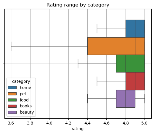
sns.boxplot(df_products, x='rating', hue='category', orient='h', showfliers=False)
plt.title('Rating range by category')
plt.grid()
plt.show()
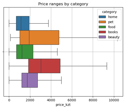
sns.boxplot(df_products, x='price_kzt', hue='category', orient='h', showfliers=False)
plt.title('Price ranges by category')
plt.grid()
plt.show()
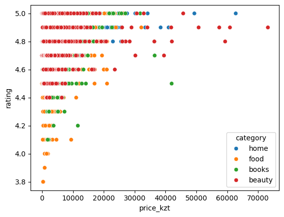
sns.scatterplot(df_products, x='price_kzt', y='rating', hue='category')
plt.show()
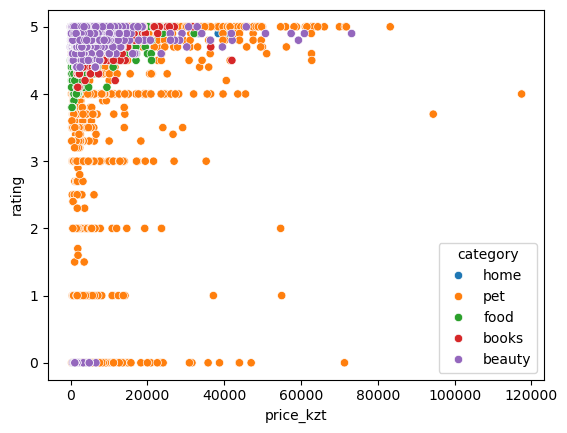
Price–Rating Correlation by Category
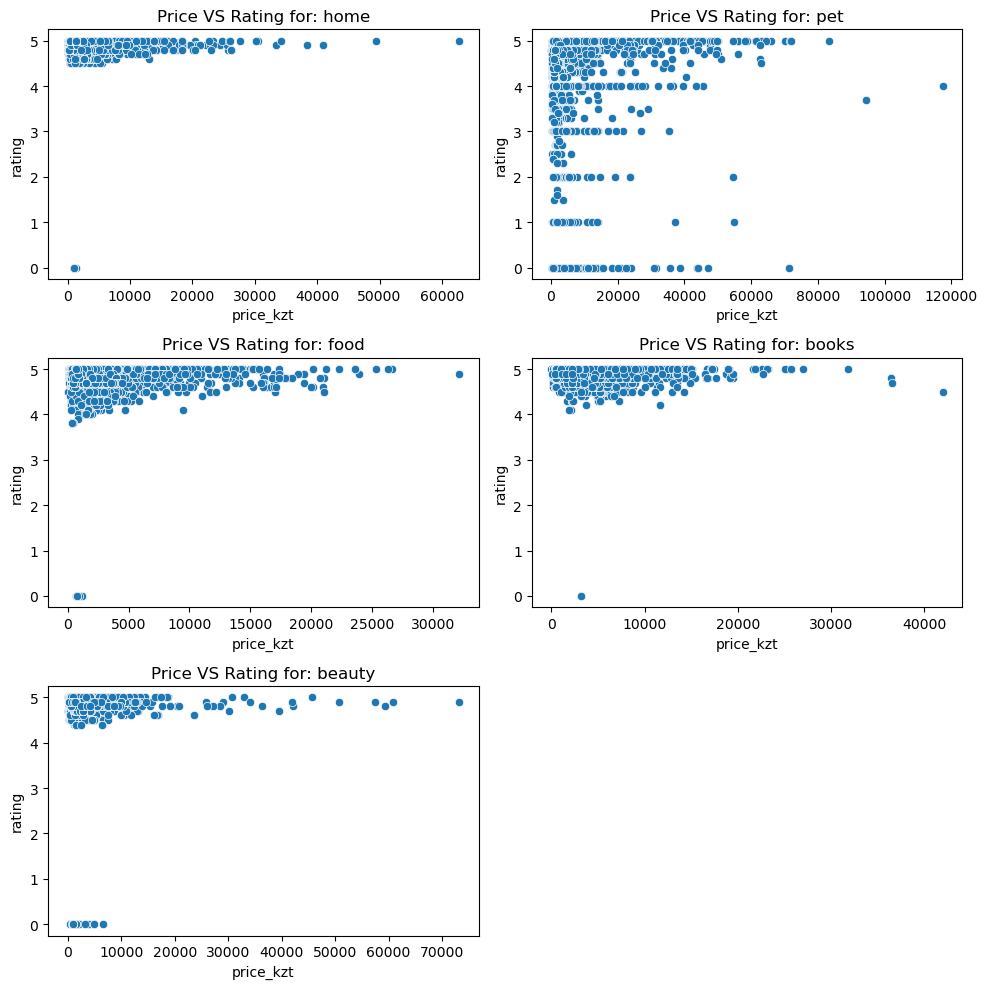
Price–Rating Correlation (Excluding Pet Products)
sns.scatterplot(df_products[(df_products['category']!='pet')&(df_products['rating']>3)], x='price_kzt', y='rating', hue='category')
plt.show()
Books#
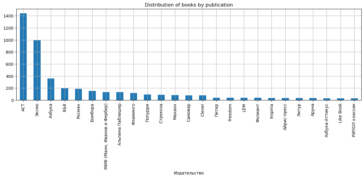
Distribution of books by publication
df_books['Издательство'].value_counts().head(25).plot(kind='bar', figsize=(15, 4))
plt.title('Distribution of books by publication')
plt.grid()
plt.show()
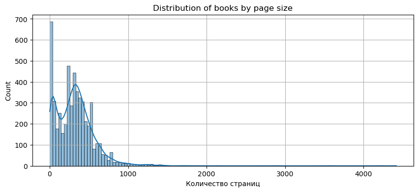
Distribution of books by page size
plt.figure(figsize=(10, 4))
sns.histplot(data=df_books, x='Количество страниц', kde=True)
plt.title('Distribution of books by page size')
plt.grid()
plt.show()
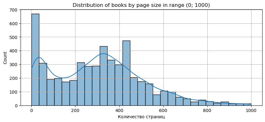
plt.figure(figsize=(10, 4))
sns.histplot(data=df_books[df_books['Количество страниц']<=1000], x='Количество страниц', kde=True, stat='count')
plt.title('Distribution of books by page size in range (0; 1000)')
plt.grid()
plt.show()
Distribution of the books based on the language
df_books['Язык'].dropna().str.split(',').explode().str.strip().value_counts()
Язык
русский        5264
казахский       153
английский       96
немецкий          5
корейский         3
турецкий          2
японский          2
итальянский       1
испанский         1
грузинский        1
белорусский       1
Name: count, dtype: int64
Distribution of the books based on paper type
df_books['Бумага'].value_counts()
Бумага
офсетная                   1933
газетная                    816
типографская                271
офсетная, пухлая            187
мелованная                  154
пухлая, типографская        126
картон                       34
газетная, пухлая             33
пухлая                       26
ламинированные               14
кремовый офсет               13
тонированная                  7
глянцевая                     5
офсетная, мелованная          4
creamy пухлая                 3
матовая, мелованная           3
классик                       2
ПВХ                           2
белая                         2
creamy пухлая, офсетная       1
дизайнерская бумага           1
мелованная, офсетная          1
мелованная, матовая           1
кремовый офсет, пухлая        1
Name: count, dtype: int64
Pairwise Correlation of Numerical Variables
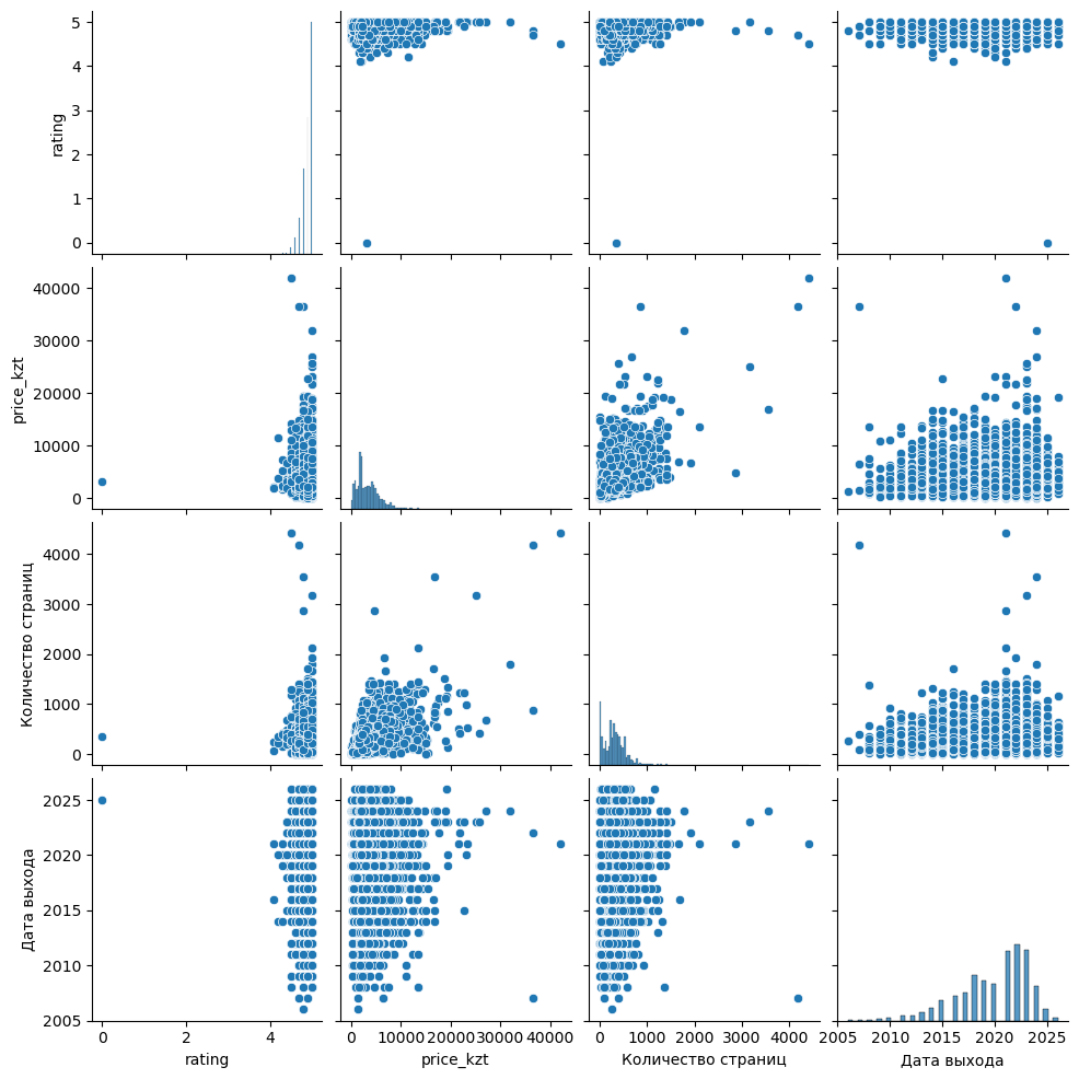
sns.pairplot(df_books.drop(columns=['id']))
plt.show()
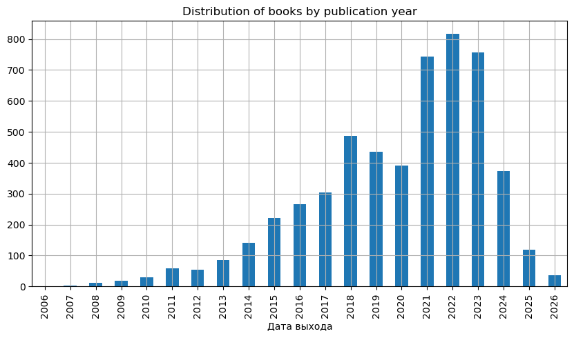
Distribution of books by publication year
df_books['Дата выхода'].value_counts().sort_index().plot(kind='bar', figsize=(10, 5))
plt.title('Distribution of books by publication year')
plt.grid()
plt.show()
AI-Summary Tags Analysis#
from wordcloud import WordCloud
positive_tags = df_products['ai_positive_tags'].explode().dropna().astype(str).tolist()
negative_tags = df_products['ai_negative_tags'].explode().dropna().astype(str).tolist()
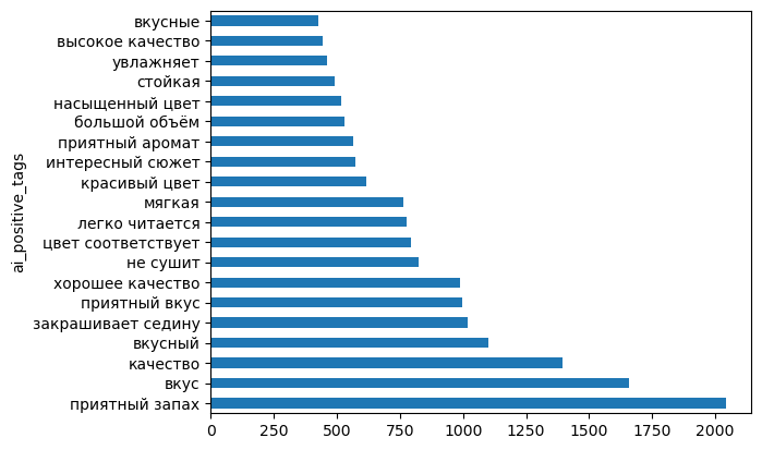
Positive Tag Distribution (Top 20)
df_products['ai_positive_tags'].explode().value_counts().head(20).plot(kind='barh')
plt.show()
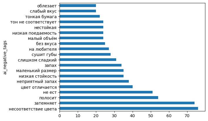
Negative Tag Distribution (Top 20)
df_products['ai_negative_tags'].explode().value_counts().head(20).plot(kind='barh')
plt.show()
Positive Tags Word Cloud Analysis
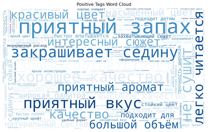
Negative Tags Word Cloud Analysis
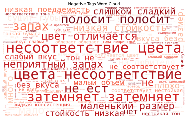
Positive vs Negative Tags Word Cloud
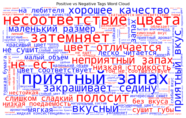
Positive Tag Frequency by Category
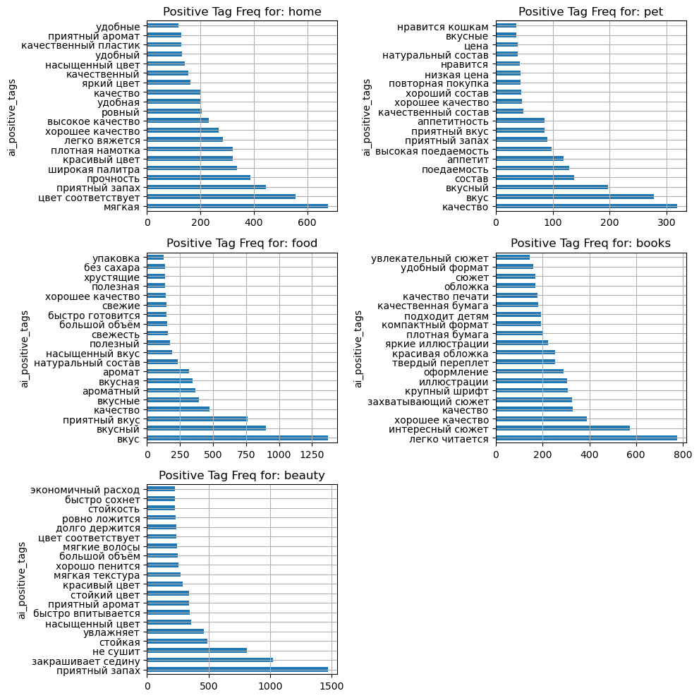
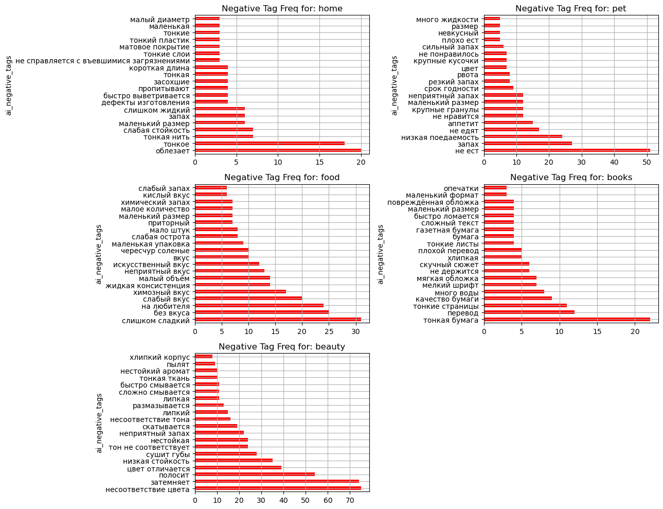
Negative Tag Frequency by Category
Voice of Customer (VoC) & Root Cause Analysis#
There used AI summaries and review tags to identify root causes of customer dissatisfaction, prioritized issues by business impact.
from pymorphy3 import MorphAnalyzer
from sentence_transformers import SentenceTransformer, util
df_reviews = pd.read_csv('data/product_reviews.csv', index_col=False)
df_reviews = df_reviews.copy().reset_index(names='id')
df_reviews.info()
<class 'pandas.core.frame.DataFrame'>
RangeIndex: 431043 entries, 0 to 431042
Data columns (total 8 columns):
 #   Column      Non-Null Count   Dtype
---  ------      --------------   -----
 0   id          431043 non-null  int64
 1   product_id  431043 non-null  int64
 2   date        431043 non-null  object
 3   author      426859 non-null  object
 4   rating      431043 non-null  float64
 5   pros        200352 non-null  object
 6   cons        143392 non-null  object
 7   text        398765 non-null  object
dtypes: float64(1), int64(2), object(5)
memory usage: 26.3+ MB
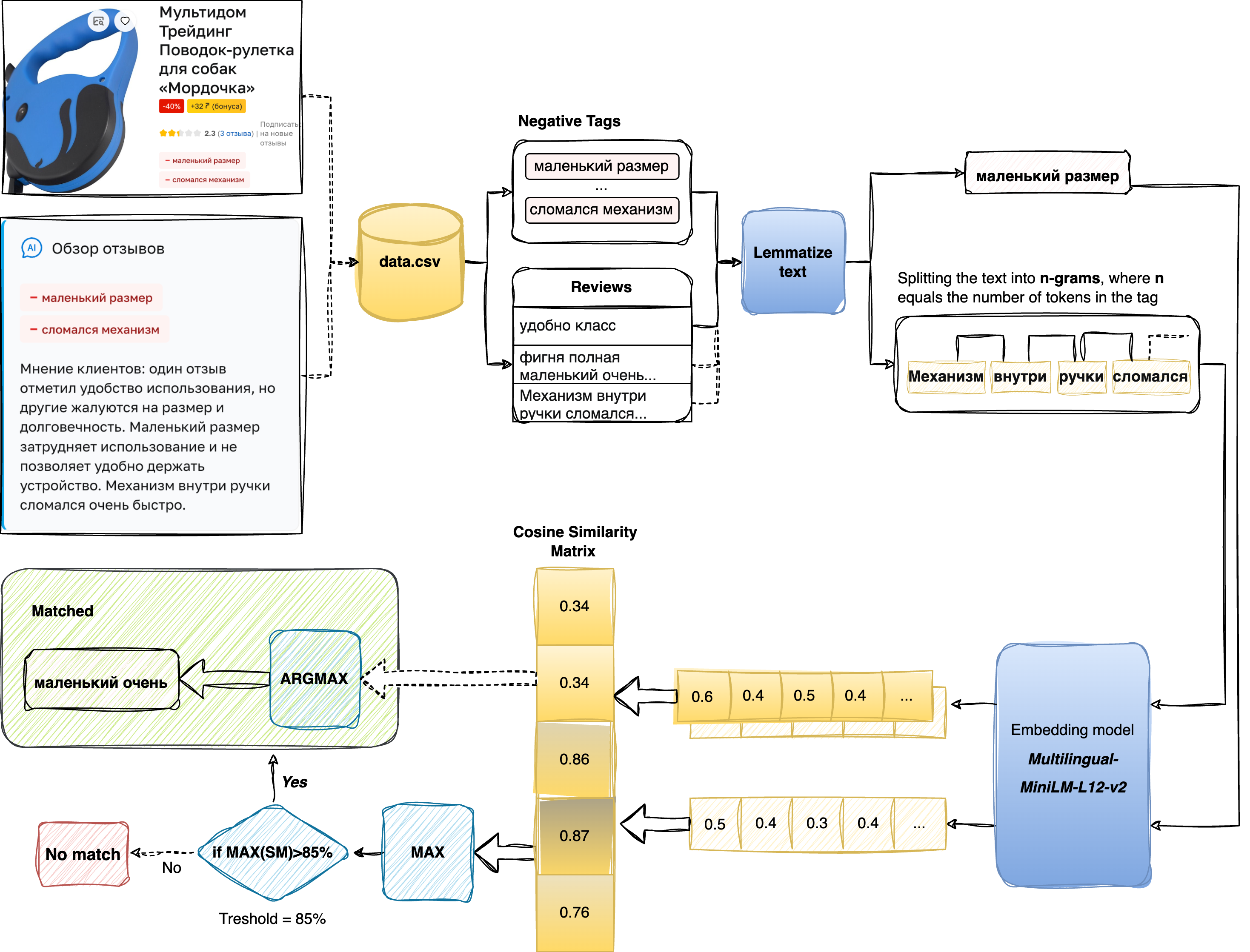
We propose a practical approach to RCA and Voice of Customer analysis when raw review labeling is unavailable, but AI generated summaries and positive/negative tags are already available. This provides a strong foundation for identifying product issues, although access to richer data, such as sales, returns, or operational metrics would allow for a more advanced analysis.
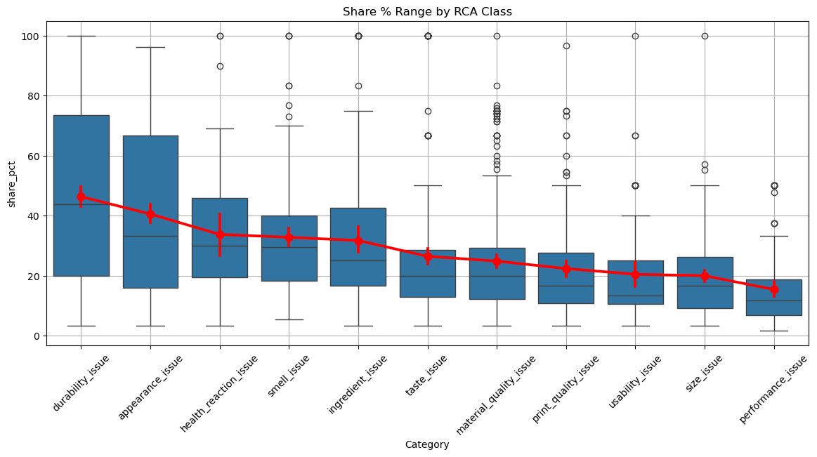
Our dataset includes product information and customer reviews. For each product with negative tags, we estimate the share of each problem. First both review texts and negative tags are cleaned and lemmatized. Each review is then split into n-grams, where n equals the length of the tag being matched. Next we use the paraphrase-multilingual-MiniLM-L12-v2 (emb size = 384) embedding model to encode both tags and review chunks. Cosine similarity is calculated between each tag embedding and the embeddings of review chunks, producing a similarity matrix.
If the maximum similarity exceeds a predefined threshold the tag is considered detected in that review, otherwise it is treated as not matched. Using argmax we can also identify the review chunk that is most similar to the tag. Based on these matches we calculate the share of each negative tag within a product reviews. This metric helps rank issues in the RCA analysis and identify the most prominent customer pain points.
Finally, similar tags can be clustered into broader problem groups, which supports higher-level RCA categorization and allows issues to be ranked by severity, for example as low, high, or critical.
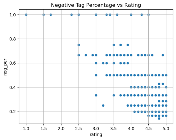
Negative Tag Percentage vs Rating
Text Cleaning and Preprocessing#
morph = MorphAnalyzer()
NEGATIONS = {'не', 'ни', 'нет'}


def clean_text(text: str) -> str:
    if pd.isna(text):
        return ''
    text = str(text).lower().strip()
    text = re.sub(r'[^а-яёa-z0-9\s]', ' ', text) #leave only text and numbers
    text = re.sub(r'\s+', ' ', text).strip() #removing extra spaces
    return text


#negations are an important part of text analysis. In our case we join negation
# with the following word using an underscore to avoid splitting negated expressions when generating n-grams
def bind_negations(tokens: list[str]) -> list[str]:
    bound = []
    i = 0

    while i < len(tokens):
        if tokens[i] in NEGATIONS and i + 1 < len(tokens):
            bound.append(f'{tokens[i]}_{tokens[i + 1]}')
            i += 2
        else:
            bound.append(tokens[i])
            i += 1

    return bound


def lemmatize(text: str) -> list[str]:
    text = clean_text(text)
    if not text:
        return []

    words = text.split()
    lemmas = [morph.parse(w)[0].normal_form for w in words]
    lemmas = bind_negations(lemmas)

    return lemmas


def lemmatize_text(text: str) -> str:
    return ' '.join(lemmatize(text))
mask = df_products['ai_negative_tags'].notna() #products with neg tags
df_products.loc[mask, 'tag_lemma'] = df_products.loc[mask, 'ai_negative_tags'].apply(
    lambda tags: [lemmatize_text(tag) for tag in tags if tag]
)
def merge_text(*args):
    return ' '.join(
        str(arg) for arg in args
        if pd.notna(arg) and str(arg).strip()
    )

review_mask = df_reviews['product_id'].isin(df_products[mask]['id']) #reviews where products have neg tags
df_reviews.loc[review_mask, 'full_text'] = df_reviews[review_mask].apply(
    lambda row: merge_text(row['cons'], row['pros'], row['text']), axis=1
)

tqdm.pandas()
df_reviews.loc[review_mask, 'review_lemma_text'] = df_reviews.loc[review_mask, 'full_text'].progress_apply(
    lambda x: lemmatize_text(x)
)
merged = df_reviews.merge(
    df_products[~df_products['tag_lemma'].isna()][['id', 'tag_lemma']],
    left_on='product_id',
    right_on='id',
    how='right',
    suffixes=('', '_')
)
merged = merged.drop('id_', axis=1)
Tag-to-Review Similarity Matching#
minilm_model = SentenceTransformer('paraphrase-multilingual-MiniLM-L12-v2')

def n_grams(text: str, n: int) -> list[str]:
    words = str(text).split()
    if len(words) < n:
        return [str(text).strip()] if str(text).strip() else []

    windows = [
        ' '.join(words[i:i + n])
        for i in range(len(words) - n + 1)
    ]
    return list(dict.fromkeys(w.replace('_', ' ') for w in windows))

def match_tags_in_review(
    review_lemma_text: str,
    tag_lemmas: list[str],
    threshold: float = 0.85
) -> list[str]:
    if not review_lemma_text or not isinstance(tag_lemmas, list):
        return []

    review_lemma_text = str(review_lemma_text).strip()
    clean_tags = [tag.strip() for tag in tag_lemmas if isinstance(tag, str) and tag.strip()]

    if not review_lemma_text or not clean_tags:
        return []

    matched = []

    for tag in clean_tags:
        n = len(tag.split()) #window size
        grams = n_grams(review_lemma_text, n=n)

        if not grams:
            continue

        texts = [tag] + grams
        embs = minilm_model.encode(texts, normalize_embeddings=True)
        tag_emb = embs[0]
        gram_embs = embs[1:]

        sims = util.cos_sim(tag_emb, gram_embs)[0]
        best_score = float(sims.max())

        if best_score >= threshold:
            matched.append(tag)

    return list(dict.fromkeys(matched))
tqdm.pandas()
merged['matched_tags'] = merged.progress_apply(
    lambda row: match_tags_in_review(row['review_lemma_text'], row['tag_lemma']),
    axis=1
)
Callculate Share of Negative Tags
\(p\) - product
\(t\) - tag
\(R_p\) - all reviews of product \(p\)
\(e_t\) - embedding of tag \(t\)
\(e_c\) - embedding of chunk \(c\)
review_count = (
    merged.groupby('product_id', as_index=False)
    .size()
    .rename(columns={'size': 'review_count'})
)

tag_mentions = merged[['product_id', 'id', 'matched_tags']].explode('matched_tags')
tag_mentions = tag_mentions[tag_mentions['matched_tags'].notna()].copy()
tag_mentions = tag_mentions[tag_mentions['matched_tags'].astype(str).str.strip() != '']

tag_frequency = (
    tag_mentions
    .drop_duplicates(['product_id', 'id', 'matched_tags'])
    .groupby(['product_id', 'matched_tags'], as_index=False)
    .size()
    .rename(columns={
        'matched_tags': 'tag_lemma',
        'size': 'frequency'
    })
)
tag_frequency = tag_frequency.merge(review_count, on='product_id', how='left')

tag_frequency['share_pct'] = (
    tag_frequency['frequency'] / tag_frequency['review_count'] * 100
).round(1)

tag_frequency = tag_frequency.sort_values(
    ['product_id', 'frequency'],
    ascending=[True, False]
)

tag_frequency = tag_frequency.merge(
    df_products[['id', 'name', 'category', 'rating', 'price_kzt']],
    left_on='product_id',
    right_on='id',
    how='left'
)[['product_id', 'name', 'category', 'rating', 'price_kzt', 'tag_lemma', 'frequency', 'review_count', 'share_pct', ]]
tag_frequency.to_csv('data/tag_frequency.csv', index=False)
tag_frequency.info()
<class 'pandas.core.frame.DataFrame'>
RangeIndex: 2136 entries, 0 to 2135
Data columns (total 9 columns):
 #   Column        Non-Null Count  Dtype
---  ------        --------------  -----
 0   product_id    2136 non-null   int64
 1   name          2136 non-null   object
 2   category      2136 non-null   object
 3   rating        2136 non-null   float64
 4   price_kzt     2136 non-null   float64
 5   tag_lemma     2136 non-null   object
 6   frequency     2136 non-null   int64
 7   review_count  2136 non-null   int64
 8   share_pct     2136 non-null   float64
dtypes: float64(3), int64(3), object(3)
memory usage: 150.3+ KB
tag_frequency.sort_values(['share_pct'], ascending=False).head(15)
| product_id | name | category | rating | price_kzt | tag_lemma | frequency | review_count | share_pct | |
|---|---|---|---|---|---|---|---|---|---|
| 2098 | 5380803 | Мнямс Корм для кошек со вкусом кролика с зелен... | pet | 3.3 | 694.0 | отказаться есть | 2 | 2 | 100.0 |
| 153 | 731714 | Вертлюг разборный №3, большой | pet | 4.0 | 1864.0 | зазор | 2 | 2 | 100.0 |
| 592 | 1450125 | Citoderm Мыло дерматологическое для собак и кошек | pet | 4.4 | 1146.0 | запах дегтярный | 2 | 2 | 100.0 |
| 2083 | 5296803 | Caffè Borbone Кофе в капсулах со сливочным вку... | food | 4.6 | 2162.0 | растворимый кофе | 4 | 4 | 100.0 |
| 1974 | 4343595 | Faenbei Лакомство-пюре для кошек со вкусом трески | pet | 3.0 | 990.0 | отказ кот | 2 | 2 | 100.0 |
| 2084 | 5296805 | Caffè Borbone Кофе в капсулах со вкусом фундук... | food | 4.6 | 2162.0 | растворимый кофе | 4 | 4 | 100.0 |
| 2090 | 5342239 | Щетка-перчатка от шерсти животных | pet | 3.4 | 1290.0 | тряпка | 2 | 2 | 100.0 |
| 2094 | 5378122 | Мнямс Корм для кошек со вкусом говядины с клюк... | pet | 3.3 | 694.0 | отказаться есть | 2 | 2 | 100.0 |
| 1544 | 2760381 | Верный друг Присыпка для уборки | pet | 4.5 | 1600.0 | распыление | 2 | 2 | 100.0 |
| 1794 | 3397466 | Faenbei Набор пюре для кошек «Курица, треска, ... | pet | 4.0 | 990.0 | кушать | 2 | 2 | 100.0 |
| 2096 | 5378654 | Мнямс Корм для кошек со вкусом индейки с тыкво... | pet | 3.3 | 694.0 | отказаться есть | 2 | 2 | 100.0 |
| 904 | 1837074 | Yami-Yami Автокормушка-автопоилка | pet | 2.5 | 2912.0 | вода выливаться | 2 | 2 | 100.0 |
| 2100 | 5381294 | Мнямс Корм для кошек со вкусом лосося с яблоко... | pet | 3.3 | 694.0 | отказаться есть | 2 | 2 | 100.0 |
| 2107 | 5390803 | Мнямс Корм для кошек старше 7 лет «Кусочки в с... | pet | 4.5 | 470.0 | не_нравиться | 2 | 2 | 100.0 |
| 2106 | 5390700 | Мнямс Корм для кошек «Кусочки в соусе с форелью» | pet | 4.5 | 470.0 | не_нравиться | 2 | 2 | 100.0 |
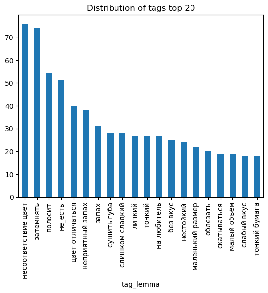
tag_frequency['tag_lemma'].value_counts().head(20).plot(kind='bar')
plt.title('Distribution of tags top 20')
plt.show()
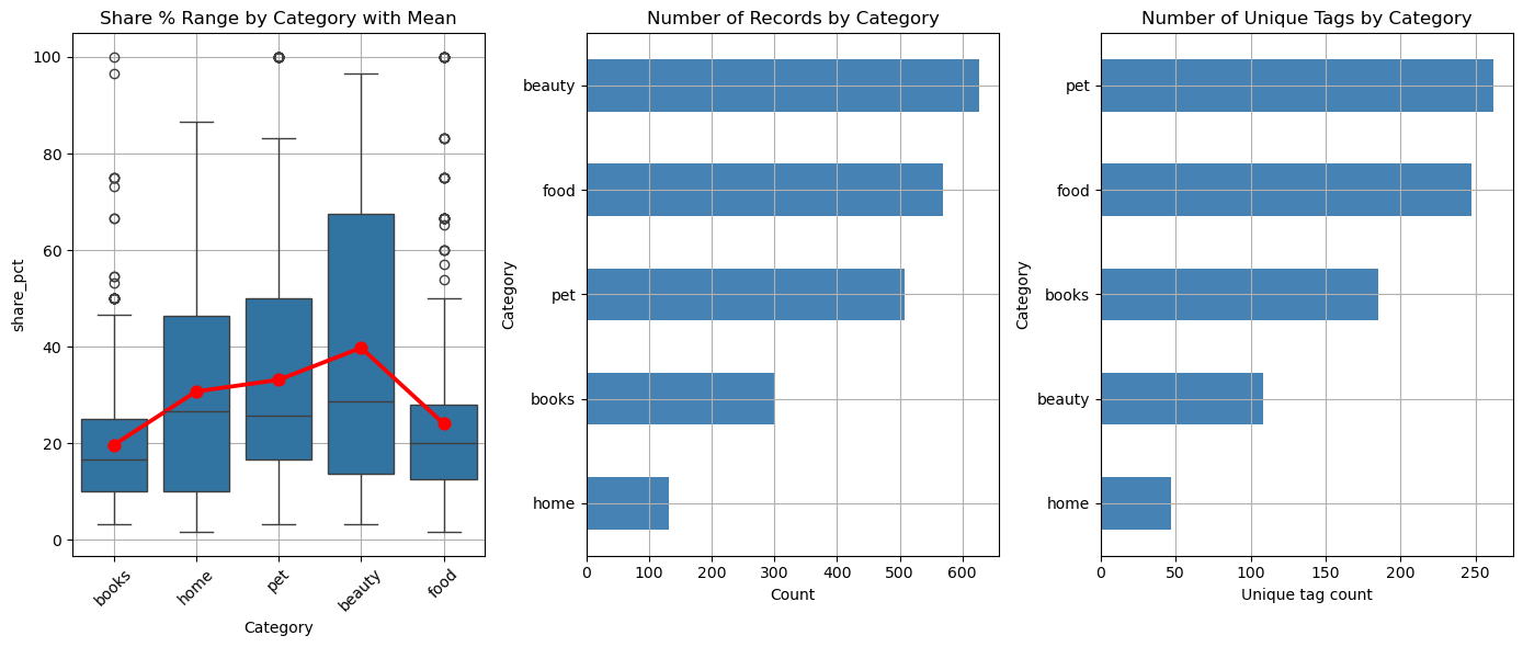
Issue Tag Classification (RCA Taxonomy)#
The next step is to cluster the main product issues. There are 733 unique keywords (neg tags), which is too many to classify manually.
tag_frequency = pd.read_csv('data/tag_frequency.csv', index_col=False)
tag_frequency.info()
<class 'pandas.core.frame.DataFrame'>
RangeIndex: 2136 entries, 0 to 2135
Data columns (total 10 columns):
 #   Column        Non-Null Count  Dtype
---  ------        --------------  -----
 0   product_id    2136 non-null   int64
 1   name          2136 non-null   object
 2   category      2136 non-null   object
 3   rating        2136 non-null   float64
 4   price_kzt     2136 non-null   float64
 5   tag_lemma     2136 non-null   object
 6   frequency     2136 non-null   int64
 7   review_count  2136 non-null   int64
 8   share_pct     2136 non-null   float64
 9   class         2136 non-null   object
dtypes: float64(3), int64(3), object(4)
memory usage: 167.0+ KB
tag_frequency[['category', 'tag_lemma']].groupby('category')['tag_lemma'].unique()
category
beauty    [крошиться, хлипкий ручка, размазываться, заби...
books     [тонкий бумага, плохой перевод, не_цветной, чё...
food      [слишком сладкий, много примесь, неравномерный...
home      [тонкий, без инструкция, крупный отверстие, ма...
pet       [царапина, боль животный, выдирать шерсть, тон...
Name: tag_lemma, dtype: object
Draft Test Set Construction#
from sklearn.metrics import adjusted_rand_score, normalized_mutual_info_score, accuracy_score, classification_report
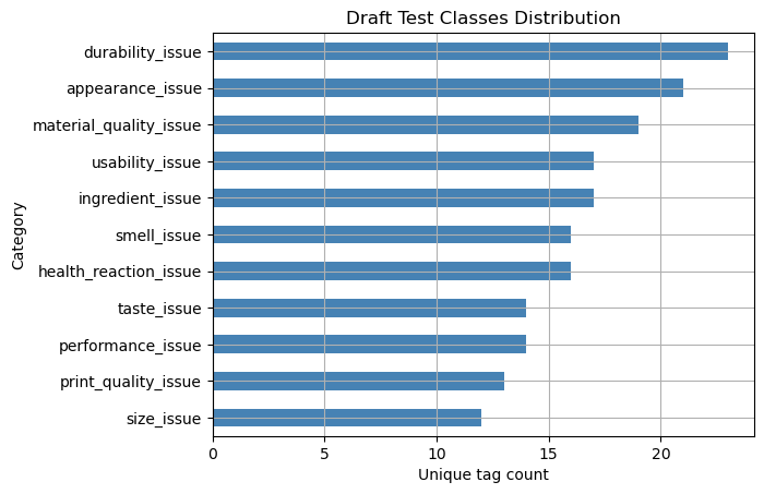
For evaluation we constructed a draft test set, where tags are manually sampled across classes.
draft_test_set = {
    'appearance_issue': [
        'белые след', 'белый налёт', 'бледный оттенок', 'жирный блеск', 'затемнять',
        'неверный оттенок', 'неверный цвет', 'неподходящий оттенок', 'краска пачкать', 'не цветной',
        'пятно', 'цвет обложка', 'чернильный пятно', 'чёрно белые картинка', 'серый цвет',
        'слабый цвет', 'тёмный', 'тёмный пятно', 'масляный текстура', 'жёлтый страница', 'старое'
    ],
    'durability_issue': [
        'быстро выветриваться', 'быстро подсыхать', 'быстро растекаться', 'крошиться', 'осыпаться',
        'отклеиваться', 'протекание', 'размокать', 'быстро ломаться', 'залом', 'засохнуть',
        'позолота стираться', 'порвать плёнка', 'потрепать', 'расклеиваться', 'ломаный лист', 'сломать',
        'засохнуть кусочек', 'вздутый банк', 'вздутый паучить', 'дата изготовление', 'просрочить', 'срок годность'
    ],
    'health_reaction_issue': [
        'аллергия', 'вызывать перхоть', 'вызывать раздражение', 'высыпание', 'жжение',
        'перхоть', 'покраснение', 'раздражение кожа', 'боль животный', 'вызывать рвота',
        'диарея', 'кашель', 'перхоть остаться', 'рвота', 'рвота у собака', 'вздутие'
    ],
    'ingredient_issue': [
        'примесь', 'гнилой зерно', 'много масло', 'много примесь', 'много соль',
        'много соус', 'много специя', 'наличие робуста', 'не из твёрдый мука', 'вкусовой добавка',
        'ингредиент', 'много кукуруза', 'много овощ', 'много пшеница', 'непонятный частица',
        'низкий мясо', 'плесень'
    ],
    'taste_issue': [
        'приторно', 'банановый вкус', 'без вкус', 'безвкусность', 'вкус недолговечный',
        'вкус странный', 'вкус сыр', 'высокий солёность', 'не по вкус', 'аппетит', 'без аппетит',
        'отказ от корм', 'прогорклый вкус', 'прогорклость'
    ],
    'smell_issue': [
        'запах спирт', 'иной аромат', 'искусственный запах', 'неприятный запах', 'нестойкий аромат',
        'резкий запах', 'резкий отдушка', 'аромат', 'без запах', 'запах', 'запах застарелость',
        'искусственный аромат', 'слабый аромат', 'слабый запах', 'запах протухший мясо',
        'прогорклый запах'
    ],
    'material_quality_issue': [
        'жёсткий щетина', 'липкий', 'липкость', 'мягкий щетина', 'тонкий ткань',
        'хлипкий корпус', 'хлипкий ручка', 'бумага', 'бумага газетный', 'газетный бумага',
        'грязный помятый', 'жёсткий окончание', 'мягкий обложка', 'мягкий переплёт', 'тонкий бумага',
        'грязный', 'жёсткость', 'наличие осадка', 'качество страница'
    ],
    'print_quality_issue': [
        'банальный сюжет', 'без иллюстрация', 'главный героиня', 'грамматический ошибка',
        'иллюстрация в середина', 'качество печать', 'неинтересный сюжет', 'неинтересный',
        'недосказанность', 'урезанный версия', 'мелкий схема', 'нечёткий шрифт', 'брак на корешок'
    ],
    'performance_issue': [
        'быстро смываться', 'впитывать средство', 'плохо смывать', 'средний перекрытие', 'тяжело смываться',
        'комковаться', 'ложиться неравномерно', 'плохо перемалывать', 'плохо подниматься',
        'плохо растворяться', 'замутнять вода', 'мутить вода', 'не впитывать', 'не комковаться'
    ],
    'size_issue': [
        'крупный блёстка', 'маленький объём', 'маленький размер', 'малый объём', 'маленький формат',
        'мало детектив', 'мало место', 'мало слово', 'крупный измельчение', 'крупный помол',
        'маленький порция', 'маленький упаковка'
    ],
    'usability_issue': [
        'без дозатор', 'не для жирный кожа', 'неудобный дозатор', 'неудобный крышка', 'неудобный тара',
        'трудно наноситься', 'трудно открываться', 'широкий горлышко', 'без плёнка', 'не для каждый',
        'неплотный крышка', 'слабый крышка', 'сложно открываться', 'без батарейка', 'без инструкция',
        'неудобный горлышко', 'бортик отсутствовать'
    ]
}

draft_test = pd.DataFrame(
    [(cls, tag) for cls, tags in draft_test_set.items() for tag in tags],
    columns=['class', 'tag_lemma']
)
draft_test['class_num'] = draft_test['class'].astype('category').cat.codes
draft_test.info()
<class 'pandas.core.frame.DataFrame'>
RangeIndex: 182 entries, 0 to 181
Data columns (total 3 columns):
 #   Column     Non-Null Count  Dtype
---  ------     --------------  -----
 0   class      182 non-null    object
 1   tag_lemma  182 non-null    object
 2   class_num  182 non-null    int8
dtypes: int8(1), object(2)
memory usage: 3.1+ KB
def evaluate_method(
    y_true: list,
    y_pred: list,
    method: str='Culstering with Embeddings',
    emb_model: str='paraphrase-multilingual-MiniLM-L12-v2',
    acc: bool=False
) -> dict:
    ari = adjusted_rand_score(y_true, y_pred)
    nmi = normalized_mutual_info_score(y_true, y_pred)

    print(f'Method: {method} | EmbModel: {emb_model}')
    print(f'ARI: {ari:.4f}')
    print(f'NMI: {nmi:.4f} \n')

    result = {
        'method': method,
        'emb_model': emb_model,
        'ARI': ari,
        'NMI': nmi
    }
    if acc:
        result['accuracy_score'] =  accuracy_score(y_true, y_pred)

    return result
Unsupervised Methods#
To construct the root cause taxonomy without labeled data, we first explored a set of unsupervised clustering methods. As embedding models, we tested paraphrase-multilingual-MiniLM-L12-v2 and BAAI/bge-m3.
Tag Embedding Clustering#
from sklearn.manifold import TSNE
from sklearn.cluster import AgglomerativeClustering

minilm_model = SentenceTransformer('paraphrase-multilingual-MiniLM-L12-v2')
bge_model = SentenceTransformer('BAAI/bge-m3')
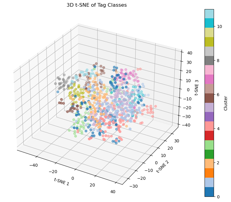
This simple method provides embeddings for these tags and then applies a clustering method to identify problem classes.
unique_tags = tag_frequency.drop_duplicates('tag_lemma').copy()
tags = unique_tags['tag_lemma'].str.replace('_', ' ', regex=False).to_list()
tag_embeddings = minilm_model.encode(
    tags,
    normalize_embeddings=True,
    show_progress_bar=True,
)
tag_embeddings_bge = bge_model.encode(
    tags,
    normalize_embeddings=True,
    show_progress_bar=True,
)
c12_model = AgglomerativeClustering(
    n_clusters=12,
    linkage='ward'
)
classes = c12_model.fit_predict(tag_embeddings)
classes_bge = c12_model.fit_predict(tag_embeddings_bge)
huggingface/tokenizers: The current process just got forked, after parallelism has already been used. Disabling parallelism to avoid deadlocks...
To disable this warning, you can either:
	- Avoid using `tokenizers` before the fork if possible
	- Explicitly set the environment variable TOKENIZERS_PARALLELISM=(true | false)
results = []

y_pred = draft_test[['tag_lemma']].merge(
    plot_df[['tag', 'class']],
    left_on='tag_lemma',
    right_on='tag',
    how='left'
)['class']
y_pred_bge = draft_test[['tag_lemma']].merge(
    pd.DataFrame({'tag':tags, 'class': classes_bge}),
    left_on='tag_lemma',
    right_on='tag',
    how='left'
)['class']

results.append(evaluate_method(
    draft_test['class_num'],
    y_pred,
    'AgglomerativeClustering with Tag Embeddings'
))
results.append(evaluate_method(
    draft_test['class_num'],
    y_pred_bge,
    'AgglomerativeClustering with Tag Embeddings',
    'BAAI/bge-m3'
))
Method: AgglomerativeClustering with Tag Embeddings | EmbModel: paraphrase-multilingual-MiniLM-L12-v2
ARI: 0.2446
NMI: 0.4571

Method: AgglomerativeClustering with Tag Embeddings | EmbModel: BAAI/bge-m3
ARI: 0.3115
NMI: 0.5252
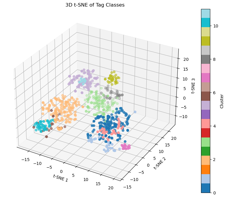
We see that clustering only using embedding is not enough accurate. Because clusters mainly capture semantic similarity, but do not form pure business categories of problems:
for class_id in sorted(plot_df['class'].unique()):
    class_tags = plot_df.loc[plot_df['class'] == class_id, 'tag'].tolist()
    print(f'\nClass {class_id} | size={len(class_tags)}')
    print(class_tags[:30])
Class 0 | size=109
['плохой перевод', 'сложно читаться', 'отсутствие аудио', 'недосказанность', 'сложный задание', 'неудачный перевод', 'некачественный переплёт', 'отсутствие диск', 'некачественный оформление', 'сложно читать', 'тяжёлый язык', 'запачканность', 'затянутость', 'боль животный', 'плохо сматываться', 'бортик плохо фиксироваться', 'много кровь', 'старорусский слово', 'тяжело читаться', 'искажённый имя', 'непонятный задание', 'неправильный буква', 'неинтересный кошка', 'подделка', 'повреждение', 'плохо приниматься', 'трудный чтение', 'раздражение кожа', 'сложно смываться', 'нестойкий']

Class 1 | size=81
['тонкий бумага', 'не цветной', 'чёрно белые страница', 'сложный текст', 'маленький формат', 'мелкий шрифт', 'тонкий карта', 'газетный бумага', 'обложка', 'мало казахстан', 'тонкий страница', 'без иллюстрация', 'черно белый печать', 'тонкий лист', 'бумага газетный', 'мало страница', 'чёрно белые картинка', 'бумага', 'карабин', 'хлипкий ручка', 'несоответствие цвет', 'иллюстрация в середина', 'качество страница', 'тёмный бумага', 'серый страница', 'маркировка', 'бумага серый', 'библейский отсылка', 'цвет отличаться', 'неровный страница']

Class 10 | size=37
['тяжёлый содержание', 'много повтор', 'крупный отверстие', 'цена', 'крупный палочка', 'много примесь', 'размер', 'больший', 'слишком больший', 'тяжёлый слог', 'высокий цена', 'крупный измельчение', 'объём', 'крупный', 'много гранула', 'крупный гранула', 'много углевод', 'дорого', 'трата деньга', 'большой объём', 'вздутый банк', 'состояние', 'крупный блёстка', 'много цифра', 'докупать', 'измельчение', 'помол крупноватый', 'большой размер', 'крупный кусочек', 'крупный кусок']

Class 11 | size=19
['много вода', 'плавать корм', 'жидкость', 'не для вода', 'не впитывать', 'не подходить для аквариум с сом', 'не пить вода', 'замутнять вода', 'мутить вода', 'жидкий консистенция', 'без батарейка', 'жидкий', 'вода выливаться', 'много жидкость', 'водянистый', 'впитывать средство', 'мутный вода', 'жидковато', 'питься тяжело']

Class 2 | size=85
['тонкий обложка', 'поверхностный информация', 'мягкий обложка', 'тонкий картон', 'хлипкий', 'некачественный пластик', 'материал', 'неоднородный стекло', 'мягкий резина', 'мусорить', 'тонкий металл', 'ржаветь', 'пылить', 'качество мех', 'жёсткий материал', 'липкий', 'стягивать кожа', 'слабый увлажнение', 'излишек продукт', 'сушить кожа', 'шерсть жёсткий', 'неравномерный обжарка', 'мягкий щетина', 'не для густой шерсть', 'много продукт', 'пересолить', 'горелый', 'твёрдый шелуха', 'солома', 'тонкий ткань']

Class 3 | size=49
['нет пример', 'не для каждый', 'не для короткошёрстный', 'не держаться', 'слишком простой', 'не восторг', 'не есть', 'не комковаться', 'не катиться', 'слишком сладкий', 'нет оттенок', 'бортик отсутствовать', 'нет новизна', 'неинтересный', 'не прочный', 'слишком твёрдый', 'без плёнка', 'не нравиться', 'чересчур сладкий', 'малосладкий', 'не окрашивать', 'не подходить', 'не есть крыса', 'слишком жидкий', 'без дозатор', 'слишком сладкое', 'не прикоснуться', 'нет зип замок', 'безвкусность', 'невкусный']

Class 4 | size=103
['качество бумага', 'типографский брак', 'скучный сюжет', 'опечатка', 'урезанный версия', 'неуказанный возраст', 'возраст завысить', 'жёсткий окончание', 'на любитель', 'научный язык', 'брак', 'сбивчивый повествование', 'чрезмерный жестокость', 'шаблонность', 'сложный восприятие', 'банальный сюжет', 'неинтересный сюжет', 'качество печать', 'незавершённый концовка', 'без инструкция', 'качество', 'быстро крошиться', 'разгрызание', 'картинка запаздывать', 'быстро рваться', 'качество обработка', 'двусторонний', 'оформление', 'скучный', 'легко гнуться']

Class 5 | size=120
['мягкий переплёт', 'сократить текст', 'пачкаться срез', 'перевод', 'порода', 'тонкий', 'царапина', 'выдирать шерсть', 'тонкий стелька', 'тонковатый', 'разваливаться', 'рваться', 'крошиться', 'тонкий крепление', 'помятый край', 'перо выпадать', 'нитка распускаться', 'зазор', 'толстой', 'размазываться', 'склеивать ресница', 'индейка', 'вздутие', 'подчёркивать морщина', 'расклеиваться', 'много болтовня', 'осыпаться', 'кривая наклейка', 'примесь', 'липнуть']

Class 6 | size=53
['позолота стираться', 'отсутствие мясо', 'подача корм', 'низкий мясо', 'банановый вкус', 'пшеничный мука', 'пальмовый масло', 'ежедневный питание', 'много кукуруза', 'много пшеница', 'плохо есть', 'похожий на кетчуп', 'кокосовый привкус', 'без аппетит', 'сушить губа', 'аппетит', 'масляный текстура', 'мало специя', 'мясной кусочек', 'постоянный кормление', 'много специя', 'с рис', 'печь губа', 'сырой', 'специя специфический', 'много соус', 'много масло', 'преобладание яблоко', 'отказ от корм', 'поедаемость']

Class 7 | size=44
['мало задание', 'мало новый', 'мало текст', 'маленький размер', 'малый количество', 'малый размер', 'малый диаметр', 'мало место', 'маленький', 'недолговечный', 'мало резьба', 'жирность', 'краткость изложение', 'маленький объём', 'малый объём', 'маленький упаковка', 'короткий', 'малый вес', 'маленький фасовка', 'мелкий шарик', 'мелкий помол', 'малый порция', 'мелкий крупа', 'мало порция', 'мало', 'мелкий хлебец', 'маленький порция', 'несоответствие размер', 'редкий кусочек', 'короткий длина']

Class 8 | size=33
['химический запах', 'запах', 'горелый запах', 'неприятный запах', 'резкий запах', 'нестойкий запах', 'запах резина', 'сильный запах', 'слабый запах', 'слабый аромат', 'специфический запах', 'искусственный запах', 'запах застарелость', 'запах дегтярный', 'плохой запах', 'резковатый запах', 'не впитывать запах', 'мятный запах', 'искусственный аромат', 'сильный ароматизатор', 'запах спирт', 'неудержание запах', 'короткий срок запах', 'тяжёлый запах', 'запах книга', 'неприятный аромат', 'без запах', 'запах протухший мясо', 'аромат', 'нестойкий аромат']

Class 9 | size=40
['вкус', 'не по вкус', 'менять вкус', 'слабый вкус', 'горький привкус', 'химозный вкус', 'искусственный вкус', 'горький вкус', 'непривычный привкус', 'вкус странный', 'горьковатый вкус', 'посторонний привкус', 'неприятный вкус', 'кислый вкус', 'не вкусный', 'ржаный привкус', 'вкус не для весь', 'усилитель вкус', 'без вкус', 'вкус недолговечный', 'неравномерный вкус', 'специфический вкус', 'несоответствие вкус', 'изменчивый вкус', 'странный вкус', 'неприятный привкус', 'некофейный вкус', 'прогорклый вкус', 'нет вкус', 'непонятный вкус']
Tag + Category Embedding Clustering#
tag_cat_pairs = (
    unique_tags['category'] + ': ' +
    unique_tags['tag_lemma'].str.replace('_', ' ', regex=False)
).tolist()

tag_cat_embeddings = minilm_model.encode(
    tag_cat_pairs,
    normalize_embeddings=True,
    show_progress_bar=True,
)

tag_cat_embeddings_bge = bge_model.encode(
    tag_cat_pairs,
    normalize_embeddings=True,
    show_progress_bar=True,
)
y_pred = draft_test[['tag_lemma']].merge(
    plot_df[['tag', 'class']],
    left_on='tag_lemma',
    right_on='tag',
    how='left'
)['class']
y_pred_bge = draft_test[['tag_lemma']].merge(
    pd.DataFrame({'tag':tags, 'class': classes_bge}),
    left_on='tag_lemma',
    right_on='tag',
    how='left'
)['class']

results.append(evaluate_method(
    draft_test['class_num'],
    y_pred,
    'AgglomerativeClustering with Tag + Category Embedding'
))
results.append(evaluate_method(
    draft_test['class_num'],
    y_pred_bge,
    'AgglomerativeClustering with Tag + Category Embedding',
    'BAAI/bge-m3'
))
Method: AgglomerativeClustering with Tag + Category Embedding | EmbModel: paraphrase-multilingual-MiniLM-L12-v2
ARI: 0.0943
NMI: 0.3491

Method: AgglomerativeClustering with Tag + Category Embedding | EmbModel: BAAI/bge-m3
ARI: 0.0943
NMI: 0.3491
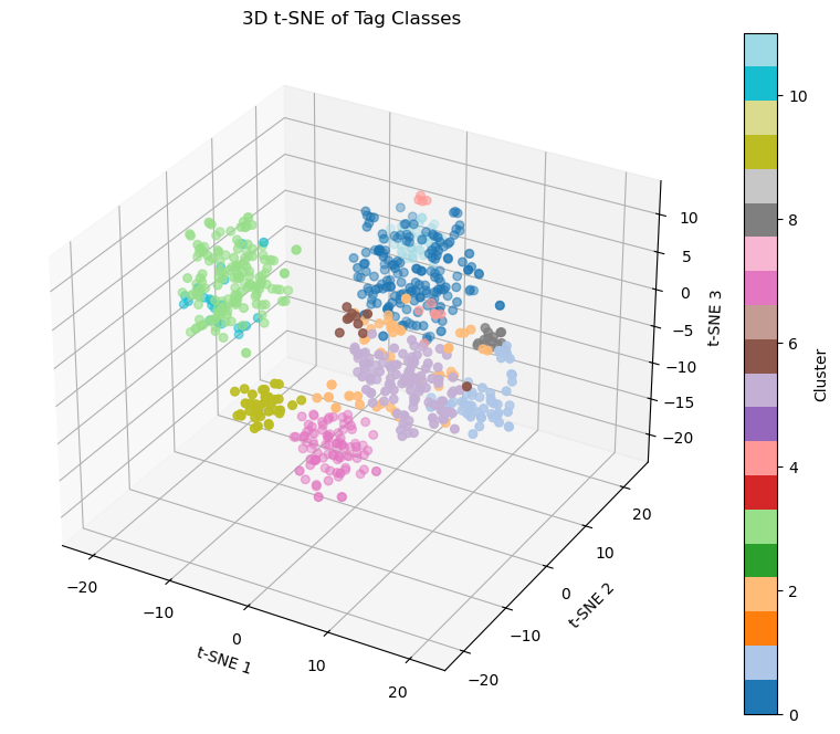
When category information was directly added to tag text embeddings, clustering quality increased in terms of category separation, but the resulting clusters became dominated by product category rather than problem type. This suggests that category aware embeddings are useful for within category analysis, but less suitable for building a global RCA taxonomy across categories.
Tag Embedding + One-Hot Category Features#
cat_one_hot = pd.get_dummies(unique_tags['category']).astype(float)
print('For MiniLM-L12-v2 Embeddings:')
print(tag_embeddings.shape,'+', cat_one_hot.shape)
merged_embeddings = np.concatenate([tag_embeddings, cat_one_hot], axis=1)
print('=', merged_embeddings.shape, '\n')

print('For bge-m3 Embeddings:')
print(tag_embeddings_bge.shape,'+', cat_one_hot.shape)
merged_embeddings_bge = np.concatenate([tag_embeddings_bge, cat_one_hot], axis=1)
print('=', merged_embeddings_bge.shape)
For MiniLM-L12-v2 Embeddings:
(773, 384) + (773, 5)
= (773, 389)

For bge-m3 Embeddings:
(773, 1024) + (773, 5)
= (773, 1029)
y_pred = draft_test[['tag_lemma']].merge(
    plot_df[['tag', 'class']],
    left_on='tag_lemma',
    right_on='tag',
    how='left'
)['class']
y_pred_bge = draft_test[['tag_lemma']].merge(
    pd.DataFrame({'tag':tags, 'class': classes_bge}),
    left_on='tag_lemma',
    right_on='tag',
    how='left'
)['class']

results.append(evaluate_method(
    draft_test['class_num'],
    y_pred,
    'AgglomerativeClustering with Tag + One Hot Cat Embedding'
))
results.append(evaluate_method(
    draft_test['class_num'],
    y_pred_bge,
    'AgglomerativeClustering with Tag + One Hot Cat Embedding',
    'BAAI/bge-m3'
))
Method: AgglomerativeClustering with Tag + One Hot Cat Embedding | EmbModel: paraphrase-multilingual-MiniLM-L12-v2
ARI: 0.1094
NMI: 0.3706

Method: AgglomerativeClustering with Tag + One Hot Cat Embedding | EmbModel: BAAI/bge-m3
ARI: 0.1043
NMI: 0.3570
We still observe the same issue as in previous method, but with slightly better metrics, as category embeddings do not have a significant impact compared to the prev method.
Semi-Supervised Methods#
Nearest-Anchor Similarity (assign class = max similarity anchor)#
The classification method works as follows:
For each input tag, we compute its embedding and measure similarity against all anchor embeddings.
The tag is then assigned to the class of the most similar anchor.
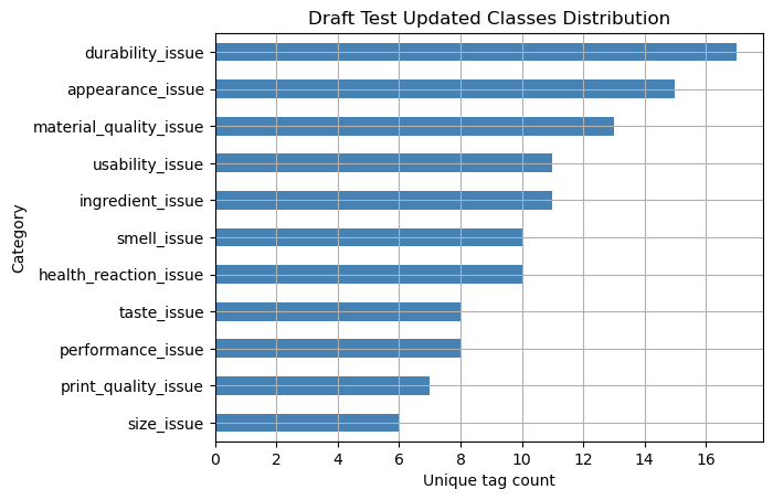
The anchor set consists of prelabled tags grouped into known classes. For each class we also build a draft anchor set, where we randomly sample a small number of representative tags (6 per class). These anchors are intended to capture the core semantics of each class without introducing too much repetition.
anchor_tags = draft_test.groupby('class')[['class', 'class_num', 'tag_lemma']].apply(
    lambda x: x.sample(6, random_state=41),
).reset_index(drop=True)
anchor_tags = anchor_tags.sample(frac=1, random_state=41).reset_index(drop=True)

draft_test_updated = draft_test[~draft_test['tag_lemma'].isin(anchor_tags['tag_lemma'])]
# for a fair test we remove tags that already exist in the anchor set
anchor_tags.head(10)
| class | class_num | tag_lemma | |
|---|---|---|---|
| 0 | size_issue | 7 | крупный помол |
| 1 | print_quality_issue | 6 | иллюстрация в середина |
| 2 | appearance_issue | 0 | цвет обложка |
| 3 | print_quality_issue | 6 | урезанный версия |
| 4 | taste_issue | 9 | без аппетит |
| 5 | durability_issue | 1 | залом |
| 6 | taste_issue | 9 | вкус сыр |
| 7 | usability_issue | 10 | неплотный крышка |
| 8 | size_issue | 7 | маленький формат |
| 9 | taste_issue | 9 | вкус недолговечный |
draft_test_updated.groupby('class')['tag_lemma'].nunique().sort_values().plot(
    kind='barh',
    color='steelblue'
)
plt.title('Draft Test Updated Classes Distribution')
plt.xlabel('Unique tag count')
plt.ylabel('Category')
plt.grid()
plt.show()
def predict_class_by_anchor(
    tags: list[str],
    anchor_tags: pd.DataFrame,
    emb_model: SentenceTransformer,
) -> pd.DataFrame:
    tag_embeddings = emb_model.encode(
        tags,
        normalize_embeddings=True,
        show_progress_bar=True
    )
    anchor_tag_embeddings = emb_model.encode(
        anchor_tags['tag_lemma'].to_list(),
        normalize_embeddings=True,
        show_progress_bar=True
    )

    sims = util.cos_sim(tag_embeddings, anchor_tag_embeddings)
    best_ids = np.argmax(sims, axis=1)

    return pd.DataFrame({
        'class': anchor_tags.iloc[best_ids]['class'].values,
        'class_num': anchor_tags.iloc[best_ids]['class_num'].values,
        'tag_lemma': tags,
        'matched_anchor': anchor_tags.iloc[best_ids]['tag_lemma'].values,
        'similarity': sims[np.arange(sims.shape[0]), best_ids]
    })
pred_df = predict_class_by_anchor(draft_test_updated['tag_lemma'].to_list(), anchor_tags, minilm_model)
pred_bge_df = predict_class_by_anchor(draft_test_updated['tag_lemma'].to_list(), anchor_tags, bge_model)

results.append(
    evaluate_method(
        draft_test_updated['class_num'].to_list(), pred_df['class_num'].to_list(),
        'Nearest-Anchor by Embedding', acc=True
    )
)
print(classification_report(draft_test_updated['class_num'].to_list(), pred_df['class_num'].to_list()))

results.append(
    evaluate_method(
        draft_test_updated['class_num'].to_list(), pred_bge_df['class_num'].to_list(),
        'Nearest-Anchor by Embedding',
        'BAAI/bge-m3', acc=True
    )
)
print(classification_report(draft_test_updated['class_num'].to_list(), pred_bge_df['class_num'].to_list()))
Method: Nearest-Anchor by Embedding | EmbModel: paraphrase-multilingual-MiniLM-L12-v2
ARI: 0.2418
NMI: 0.5011

              precision    recall  f1-score   support

           0       0.53      0.60      0.56        15
           1       0.32      0.53      0.40        17
           2       0.36      0.40      0.38        10
           3       0.50      0.27      0.35        11
           4       1.00      0.69      0.82        13
           5       0.36      0.50      0.42         8
           6       0.00      0.00      0.00         7
           7       0.67      1.00      0.80         6
           8       0.82      0.90      0.86        10
           9       0.80      0.50      0.62         8
          10       0.83      0.45      0.59        11

    accuracy                           0.53       116
   macro avg       0.56      0.53      0.53       116
weighted avg       0.57      0.53      0.53       116

Method: Nearest-Anchor by Embedding | EmbModel: BAAI/bge-m3
ARI: 0.4013
NMI: 0.5883

              precision    recall  f1-score   support

           0       0.62      0.67      0.65        15
           1       0.78      0.82      0.80        17
           2       0.88      0.70      0.78        10
           3       0.57      0.36      0.44        11
           4       0.73      0.62      0.67        13
           5       0.50      0.62      0.56         8
           6       0.10      0.14      0.12         7
           7       0.86      1.00      0.92         6
           8       1.00      0.70      0.82        10
           9       0.50      0.75      0.60         8
          10       0.50      0.45      0.48        11

    accuracy                           0.63       116
   macro avg       0.64      0.62      0.62       116
weighted avg       0.66      0.63      0.64       116
pred_df.head(10)
| class | class_num | tag_lemma | matched_anchor | similarity | |
|---|---|---|---|---|---|
| 0 | durability_issue | 1 | белые след | осыпаться | 0.637784 |
| 1 | durability_issue | 1 | белый налёт | осыпаться | 0.637983 |
| 2 | appearance_issue | 0 | бледный оттенок | слабый цвет | 0.739381 |
| 3 | size_issue | 7 | жирный блеск | крупный помол | 0.680680 |
| 4 | appearance_issue | 0 | неверный цвет | слабый цвет | 0.843784 |
| 5 | appearance_issue | 0 | неподходящий оттенок | неверный оттенок | 0.920777 |
| 6 | appearance_issue | 0 | краска пачкать | чернильный пятно | 0.765497 |
| 7 | appearance_issue | 0 | не цветной | слабый цвет | 0.839165 |
| 8 | appearance_issue | 0 | пятно | чернильный пятно | 0.840146 |
| 9 | appearance_issue | 0 | цвет обложка | слабый цвет | 0.750441 |
pred_bge_df.head(10)
| class | class_num | tag_lemma | matched_anchor | similarity | |
|---|---|---|---|---|---|
| 0 | appearance_issue | 0 | белые след | чернильный пятно | 0.533115 |
| 1 | material_quality_issue | 4 | белый налёт | мягкий переплёт | 0.587633 |
| 2 | appearance_issue | 0 | бледный оттенок | неверный оттенок | 0.722985 |
| 3 | ingredient_issue | 3 | жирный блеск | много масло | 0.646701 |
| 4 | appearance_issue | 0 | неверный цвет | неверный оттенок | 0.878375 |
| 5 | appearance_issue | 0 | неподходящий оттенок | неверный оттенок | 0.895321 |
| 6 | performance_issue | 5 | краска пачкать | впитывать средство | 0.590542 |
| 7 | appearance_issue | 0 | не цветной | неверный оттенок | 0.724858 |
| 8 | appearance_issue | 0 | пятно | чернильный пятно | 0.803314 |
| 9 | appearance_issue | 0 | цвет обложка | слабый цвет | 0.605489 |
Problems with this method (assign class = max similarity anchor) is if one anchor is slightly closer it dominates and nearest anchor changes class easily.
Top-k Voting Anchors#
Instead of using best anchor only, this method provides voting 3-5 top anhcors.
from collections import defaultdict

def predict_class_by_topk_weighted(
    tags: list[str],
    anchor_tags: pd.DataFrame,
    emb_model: SentenceTransformer,
    top_k: int = 5,
) -> pd.DataFrame:
    if len(anchor_tags) < top_k:
        raise TypeError('Top k should be less than count of anchor tags!')

    tag_embeddings = emb_model.encode(
        tags,
        normalize_embeddings=True,
        show_progress_bar=True
    )
    anchor_tag_embeddings = emb_model.encode(
        anchor_tags['tag_lemma'].to_list(),
        normalize_embeddings=True,
        show_progress_bar=True
    )

    sims = util.cos_sim(tag_embeddings, anchor_tag_embeddings).cpu().numpy()
    top_ids = np.argsort(sims, axis=1)[:, ::-1][:, :top_k]
    top_sims = np.take_along_axis(sims, top_ids, axis=1)
    class_scores = []
    class_evidence = []

    for ids, scores in zip(top_ids, top_sims):
        classes = anchor_tags['class_num'].values[ids]
        anchors = anchor_tags['tag_lemma'].values[ids]

        score_dict = defaultdict(float)
        evid_dict = defaultdict(list)

        for cls, sim, anchor in zip(classes, scores, anchors):
            score_dict[cls] += sim
            evid_dict[cls].append((anchor, round(float(sim), 2)))

        class_scores.append(score_dict)
        class_evidence.append(evid_dict)

    results = []

    for score_dict, evid_dict in zip(class_scores, class_evidence):
        best_class_num = max(score_dict, key=score_dict.get)
        best_class = anchor_tags[anchor_tags['class_num'] == best_class_num]['class'].iloc[0]
        best_score = score_dict[best_class_num]

        top_anchors = sorted(
            evid_dict[best_class_num],
            key=lambda x: x[1],
            reverse=True
        )

        total = sum(score_dict.values())
        confidence = score_dict[best_class_num] / total

        results.append({
            'class': best_class,
            'class_num': best_class_num,
            'score': best_score,
            'confidence': confidence,
            'top_anchors': top_anchors[:top_k]
        })

    df_results = pd.DataFrame(results)
    df_results['tag'] = tags
    return df_results
pred_df = predict_class_by_topk_weighted(draft_test_updated['tag_lemma'].to_list(), anchor_tags, minilm_model, 3)
pred_bge_df = predict_class_by_topk_weighted(draft_test_updated['tag_lemma'].to_list(), anchor_tags, bge_model, 3)

results.append(
    evaluate_method(
        draft_test_updated['class_num'].to_list(), pred_df['class_num'].to_list(),
        'Top-k voting Anchors', acc=True
    )
)
print(classification_report(draft_test_updated['class_num'].to_list(), pred_df['class_num'].to_list()))

results.append(
    evaluate_method(
        draft_test_updated['class_num'].to_list(), pred_bge_df['class_num'].to_list(),
        'Top-k voting Anchors',
        'BAAI/bge-m3', acc=True
    )
)
print(classification_report(draft_test_updated['class_num'].to_list(), pred_bge_df['class_num'].to_list()))
Method: Top-k voting Anchors | EmbModel: paraphrase-multilingual-MiniLM-L12-v2
ARI: 0.2775
NMI: 0.5221

              precision    recall  f1-score   support

           0       0.56      0.60      0.58        15
           1       0.39      0.71      0.50        17
           2       0.50      0.50      0.50        10
           3       0.50      0.27      0.35        11
           4       0.91      0.77      0.83        13
           5       0.33      0.38      0.35         8
           6       0.00      0.00      0.00         7
           7       0.67      1.00      0.80         6
           8       0.82      0.90      0.86        10
           9       0.80      0.50      0.62         8
          10       1.00      0.45      0.62        11

    accuracy                           0.57       116
   macro avg       0.59      0.55      0.55       116
weighted avg       0.60      0.57      0.56       116

Method: Top-k voting Anchors | EmbModel: BAAI/bge-m3
ARI: 0.4388
NMI: 0.6191

              precision    recall  f1-score   support

           0       0.69      0.73      0.71        15
           1       0.82      0.82      0.82        17
           2       0.80      0.80      0.80        10
           3       0.57      0.36      0.44        11
           4       0.88      0.54      0.67        13
           5       0.50      0.62      0.56         8
           6       0.09      0.14      0.11         7
           7       0.86      1.00      0.92         6
           8       1.00      0.80      0.89        10
           9       0.55      0.75      0.63         8
          10       0.45      0.45      0.45        11

    accuracy                           0.65       116
   macro avg       0.66      0.64      0.64       116
weighted avg       0.68      0.65      0.65       116
pred_df.head(10)
| class | class_num | score | confidence | top_anchors | tag | |
|---|---|---|---|---|---|---|
| 0 | durability_issue | 1 | 0.637784 | 0.345273 | [(осыпаться, 0.64)] | белые след |
| 1 | durability_issue | 1 | 0.637983 | 0.341188 | [(осыпаться, 0.64)] | белый налёт |
| 2 | appearance_issue | 0 | 0.739381 | 0.346011 | [(слабый цвет, 0.74)] | бледный оттенок |
| 3 | size_issue | 7 | 0.680680 | 0.345971 | [(крупный помол, 0.68)] | жирный блеск |
| 4 | appearance_issue | 0 | 1.442583 | 0.734974 | [(слабый цвет, 0.84), (чернильный пятно, 0.6)] | неверный цвет |
| 5 | appearance_issue | 0 | 0.920777 | 0.371489 | [(неверный оттенок, 0.92)] | неподходящий оттенок |
| 6 | appearance_issue | 0 | 1.520413 | 0.710853 | [(чернильный пятно, 0.77), (слабый цвет, 0.75)] | краска пачкать |
| 7 | appearance_issue | 0 | 0.839165 | 0.412334 | [(слабый цвет, 0.84)] | не цветной |
| 8 | appearance_issue | 0 | 0.840146 | 0.341304 | [(чернильный пятно, 0.84)] | пятно |
| 9 | appearance_issue | 0 | 1.469452 | 0.714820 | [(слабый цвет, 0.75), (чернильный пятно, 0.72)] | цвет обложка |
pred_bge_df.head(10)
| class | class_num | score | confidence | top_anchors | tag | |
|---|---|---|---|---|---|---|
| 0 | appearance_issue | 0 | 1.539604 | 1.000000 | [(чернильный пятно, 0.53), (неверный оттенок, ... | белые след |
| 1 | appearance_issue | 0 | 1.133981 | 0.658673 | [(тёмный, 0.57), (жёлтый страница, 0.56)] | белый налёт |
| 2 | appearance_issue | 0 | 2.061123 | 1.000000 | [(неверный оттенок, 0.72), (слабый цвет, 0.7),... | бледный оттенок |
| 3 | ingredient_issue | 3 | 0.646701 | 0.357700 | [(много масло, 0.65)] | жирный блеск |
| 4 | appearance_issue | 0 | 1.598488 | 0.715987 | [(неверный оттенок, 0.88), (слабый цвет, 0.72)] | неверный цвет |
| 5 | appearance_issue | 0 | 1.622366 | 0.691236 | [(неверный оттенок, 0.9), (слабый цвет, 0.73)] | неподходящий оттенок |
| 6 | performance_issue | 5 | 0.590542 | 0.346217 | [(впитывать средство, 0.59)] | краска пачкать |
| 7 | appearance_issue | 0 | 1.426581 | 0.678151 | [(неверный оттенок, 0.72), (слабый цвет, 0.7)] | не цветной |
| 8 | appearance_issue | 0 | 1.428046 | 0.702793 | [(чернильный пятно, 0.8), (затемнять, 0.62)] | пятно |
| 9 | appearance_issue | 0 | 1.184852 | 0.664475 | [(слабый цвет, 0.61), (неверный оттенок, 0.58)] | цвет обложка |
We see that this method performs better, because of top k voting. While previous method one anchor might be randomly be more similar than others and class might be misslead. BAAI/bge-m3 model actually works better, better semantic smoothing, better aligns on low resource classes and better generalize noisy tags.
Linear Support Vector Classifier (LinearSVC)#
import joblib
from sklearn.svm import LinearSVC
X_train = minilm_model.encode(
    anchor_tags['tag_lemma'].to_list(),
    normalize_embeddings=True,
    show_progress_bar=True,
)
X_test = minilm_model.encode(
    draft_test_updated['tag_lemma'].to_list(),
    normalize_embeddings=True,
    show_progress_bar=True,
)
X_train_bge = bge_model.encode(
    anchor_tags['tag_lemma'].to_list(),
    normalize_embeddings=True,
    show_progress_bar=True,
)
X_test_bge = bge_model.encode(
    draft_test_updated['tag_lemma'].to_list(),
    normalize_embeddings=True,
    show_progress_bar=True,
)
y_train = anchor_tags['class_num'].to_numpy()
y_test = draft_test_updated['class_num'].to_numpy()

print(X_train.shape, y_train.shape, X_test.shape, y_test.shape)
print(X_train_bge.shape, y_train.shape, X_test_bge.shape, y_test.shape)
(66, 384) (66,) (116, 384) (116,)
(66, 1024) (66,) (116, 1024) (116,)
clf = LinearSVC(
    class_weight='balanced',
    max_iter=20000,
    C=5
)
clf.fit(X_train, y_train)
joblib.dump(clf, 'LinearSVC.pkl')
y_pred = clf.predict(X_test)
results.append(evaluate_method(y_test, y_pred, 'LinearSVC', acc=True))
print(classification_report(y_test, y_pred))

clf = LinearSVC(
    class_weight='balanced',
    max_iter=20000,
    C=5
)
clf.fit(X_train_bge, y_train)
joblib.dump(clf, 'LinearSVC_bge_m3.pkl')
y_pred = clf.predict(X_test_bge)
results.append(evaluate_method(y_test, y_pred, 'LinearSVC', 'BAAI/bge-m3', acc=True))
print(classification_report(y_test, y_pred))
Method: LinearSVC | EmbModel: paraphrase-multilingual-MiniLM-L12-v2
ARI: 0.3874
NMI: 0.5794

              precision    recall  f1-score   support

           0       0.68      0.87      0.76        15
           1       0.53      0.59      0.56        17
           2       0.50      0.60      0.55        10
           3       0.57      0.36      0.44        11
           4       0.71      0.77      0.74        13
           5       0.75      0.38      0.50         8
           6       0.33      0.29      0.31         7
           7       0.83      0.83      0.83         6
           8       1.00      0.90      0.95        10
           9       0.80      0.50      0.62         8
          10       0.60      0.82      0.69        11

    accuracy                           0.65       116
   macro avg       0.66      0.63      0.63       116
weighted avg       0.66      0.65      0.64       116

Method: LinearSVC | EmbModel: BAAI/bge-m3
ARI: 0.5149
NMI: 0.6742

              precision    recall  f1-score   support

           0       0.81      0.87      0.84        15
           1       0.81      0.76      0.79        17
           2       0.88      0.70      0.78        10
           3       0.83      0.45      0.59        11
           4       0.69      0.85      0.76        13
           5       0.83      0.62      0.71         8
           6       0.27      0.43      0.33         7
           7       1.00      1.00      1.00         6
           8       1.00      0.90      0.95        10
           9       0.50      0.62      0.56         8
          10       0.58      0.64      0.61        11

    accuracy                           0.72       116
   macro avg       0.75      0.71      0.72       116
weighted avg       0.76      0.72      0.73       116
LinearSVC with BAAI/bge-m3 embeddings achieved best performance, significantly outperforming MiniLM across all metrics, indicating that embedding quality is the main factor for classification performance in this task.
Few-Shot Classification using LLMs#
import dspy
from dspy.teleprompt import BootstrapFewShot
lm = dspy.LM(
    'ollama_chat/llama3.1:8b',
    api_base='http://localhost:11434',
    temperature=0.0
)
dspy.configure(lm=lm)
class Classify(dspy.Signature):
    tag = dspy.InputField()
    label = dspy.OutputField(
        desc = """
        Return exactly one label from the allowed set.

        Allowed labels:
        - appearance_issue
        - durability_issue
        - health_reaction_issue
        - ingredient_issue
        - material_quality_issue
        - performance_issue
        - print_quality_issue
        - size_issue
        - smell_issue
        - taste_issue
        - usability_issue
        """
    )

class TextClassifier(dspy.Module):
    def __init__(self):
        super().__init__()
        self.predict = dspy.Predict(Classify)

    def forward(self, tag):
        return self.predict(tag=tag)

def metric(example, pred, trace=None):
    return example.labels == pred.labels
# few-shot dataset
trainset = [
    dspy.Example(
        tag=row['tag_lemma'],
        label=row['class']
    ).with_inputs('tag')
    for _, row in anchor_tags.iterrows()
]
# optimizer = BootstrapFewShot(metric=metric)

# model = optimizer.compile(
#     TextClassifier(),
#     trainset=trainset
# )
# model.save('few_shot_clf.json')
model = TextClassifier()
model.load('few_shot_clf.json')
tqdm.pandas()
draft_test_updated.loc[:, 'y_pred'] = draft_test_updated['tag_lemma'].progress_apply(
    lambda x: model(tag=x).label
)
results.append(
    evaluate_method(
        draft_test_updated['class'],
        draft_test_updated['y_pred'],
        'Few-shot classification',
        'llama3.1:8b',
        acc=True
    )
)
print(classification_report(draft_test_updated['class'], draft_test_updated['y_pred']))
Method: Few-shot classification | EmbModel: llama3.1:8b
ARI: 0.4343
NMI: 0.6263

                        precision    recall  f1-score   support

      appearance_issue       0.57      0.80      0.67        15
      durability_issue       0.69      0.65      0.67        17
 health_reaction_issue       0.83      1.00      0.91        10
      ingredient_issue       0.79      1.00      0.88        11
material_quality_issue       0.78      0.54      0.64        13
     performance_issue       0.67      0.50      0.57         8
   print_quality_issue       0.00      0.00      0.00         7
            size_issue       0.60      0.50      0.55         6
           smell_issue       1.00      1.00      1.00        10
           taste_issue       1.00      0.38      0.55         8
       usability_issue       0.37      0.64      0.47        11

              accuracy                           0.67       116
             macro avg       0.66      0.64      0.63       116
          weighted avg       0.68      0.67      0.65       116
The LLM shows that short text classification is not well suited for models such as llama3.1:8b. It achieved average performance and outperformed all methods except LinearSVC.
Results and Model Comparison#
results_df = pd.DataFrame(results)
results_df
| method | emb_model | ARI | NMI | accuracy_score | |
|---|---|---|---|---|---|
| 0 | AgglomerativeClustering with Tag Embeddings | paraphrase-multilingual-MiniLM-L12-v2 | 0.244605 | 0.457113 | NaN |
| 1 | AgglomerativeClustering with Tag Embeddings | BAAI/bge-m3 | 0.311521 | 0.525249 | NaN |
| 2 | AgglomerativeClustering with Tag + Category Em... | paraphrase-multilingual-MiniLM-L12-v2 | 0.094290 | 0.349141 | NaN |
| 3 | AgglomerativeClustering with Tag + Category Em... | BAAI/bge-m3 | 0.094290 | 0.349141 | NaN |
| 4 | AgglomerativeClustering with Tag + One Hot Cat... | paraphrase-multilingual-MiniLM-L12-v2 | 0.109406 | 0.370567 | NaN |
| 5 | AgglomerativeClustering with Tag + One Hot Cat... | BAAI/bge-m3 | 0.104338 | 0.356963 | NaN |
| 6 | Nearest-Anchor by Embedding | paraphrase-multilingual-MiniLM-L12-v2 | 0.241782 | 0.501106 | 0.534483 |
| 7 | Nearest-Anchor by Embedding | BAAI/bge-m3 | 0.401294 | 0.588265 | 0.629310 |
| 8 | Top-k voting Anchors | paraphrase-multilingual-MiniLM-L12-v2 | 0.277546 | 0.522067 | 0.568966 |
| 9 | Top-k voting Anchors | BAAI/bge-m3 | 0.438844 | 0.619084 | 0.646552 |
| 10 | LinearSVC | paraphrase-multilingual-MiniLM-L12-v2 | 0.387449 | 0.579354 | 0.646552 |
| 11 | LinearSVC | BAAI/bge-m3 | 0.514899 | 0.674198 | 0.724138 |
| 12 | Few-shot classification | llama3.1:8b | 0.434334 | 0.626342 | 0.672414 |
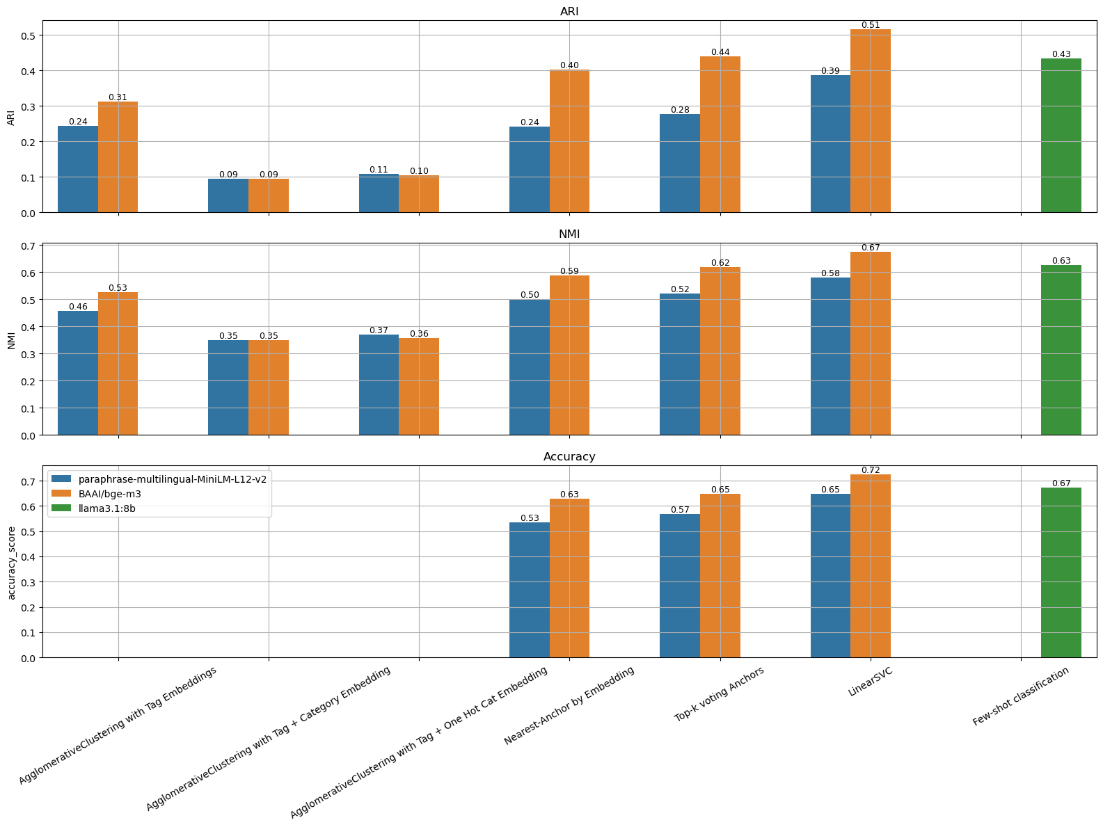
For RCA taxonomy construction, we used two approaches unsupervised and semi-supervised learning to label product issue tags. As expected, semi-supervised methods outperformed classical clustering approaches. Among semi-supervised methods, embedding based approaches consistently outperformed LinearSVC in clustering related metrics, while few-shot classification with an LLM ranked second overall. However, it outperformed LinearSVC with MiniLM (paraphrase-multilingual-MiniLM-L12-v2) (emb size 384). Overall, BGE (BAAI/bge-m3) embeddings consistently performed better than MiniLM across all methods, likely due to their higher dimensionality (emb size 1024) and stronger semantic representation capacity.
results_df.to_csv('data/results_metrics.csv')
Full Inference Pipleine#
import joblib
from pymorphy3 import MorphAnalyzer
from sentence_transformers import SentenceTransformer

emb_model = SentenceTransformer('BAAI/bge-m3')
model = joblib.load('LinearSVC_bge_m3_final.pkl')
morph = MorphAnalyzer()
rca_classes = {
    0: 'appearance_issue',
    1: 'durability_issue',
    2: 'health_reaction_issue',
    3: 'ingredient_issue',
    4: 'material_quality_issue',
    5: 'performance_issue',
    6: 'print_quality_issue',
    7: 'size_issue',
    8: 'smell_issue',
    9: 'taste_issue',
    10: 'usability_issue'
}


def clean_text(text: str) -> str:
    if pd.isna(text):
        return ''
    text = str(text).lower().strip()
    text = re.sub(r'[^а-яёa-z0-9\s]', ' ', text)
    text = re.sub(r'\s+', ' ', text).strip()
    return text

def lemmatize(text: str) -> list[str]:
    text = clean_text(text)
    if not text:
        return []

    words = text.split()
    lemmas = [morph.parse(w)[0].normal_form for w in words]

    return lemmas

def lemmatize_text(text: str) -> str:
    return ' '.join(lemmatize(text))

def predict(tags: list[str]) -> list[str]:
    tags_lemma = [lemmatize_text(tag) for tag in tags]
    tag_embeddings = emb_model.encode(
        tags,
        normalize_embeddings=True,
        show_progress_bar=False
    )
    pred_ids = model.predict(tag_embeddings)
    pred_labels = [rca_classes[i] for i in pred_ids]

    return pred_labels
predict(['плохой вкус', 'плохая упаковка'])
['taste_issue', 'usability_issue']
Business Impact Scoring#
tag_frequency = pd.read_csv('data/tag_frequency.csv', index_col=False)
tag_frequency['class'] = predict(tag_frequency['tag_lemma'].to_list())
tag_frequency.head(10)
| product_id | name | category | rating | price_kzt | tag_lemma | frequency | review_count | share_pct | class | |
|---|---|---|---|---|---|---|---|---|---|---|
| 0 | 9359 | Уголовный кодекс Республики Казахстан | books | 5.0 | 3758.0 | тонкий бумага | 2 | 11 | 18.2 | material_quality_issue |
| 1 | 17963 | Хроники Амбера: Десять романов о Янтарном коро... | books | 4.5 | 11141.0 | плохой перевод | 2 | 17 | 11.8 | print_quality_issue |
| 2 | 18490 | Ладушки. Пальчиковые игры для малышей. Развити... | books | 4.8 | 2029.0 | не_цветной | 4 | 15 | 26.7 | appearance_issue |
| 3 | 52547 | Прописи. Пособие для детей 6-7 лет | books | 4.6 | 1411.0 | чёрно белые страница | 1 | 13 | 7.7 | appearance_issue |
| 4 | 55374 | Игры, в которые играют люди: Психология челове... | books | 4.5 | 3041.0 | сложно читаться | 3 | 18 | 16.7 | print_quality_issue |
| 5 | 73876 | Сборник задач по алгебре: учебное пособие для ... | books | 4.7 | 5852.0 | тонкий бумага | 2 | 9 | 22.2 | material_quality_issue |
| 6 | 75621 | Математика. Часть 1. Для детей 5-6 лет | books | 5.0 | 414.0 | нет_пример | 1 | 5 | 20.0 | print_quality_issue |
| 7 | 85032 | Думай и Богатей! | books | 4.7 | 3082.0 | качество бумага | 1 | 28 | 3.6 | material_quality_issue |
| 8 | 86160 | Бухгалтерский учет в организациях (учебное пос... | books | 4.8 | 6256.0 | типографский брак | 1 | 5 | 20.0 | print_quality_issue |
| 9 | 89644 | Совершенный код. Мастер-класс | books | 4.9 | 13875.0 | тонкий бумага | 1 | 5 | 20.0 | material_quality_issue |
tag_frequency.to_csv('data/tag_frequency.csv', index=False)
tag_frequency.info()
<class 'pandas.core.frame.DataFrame'>
RangeIndex: 2136 entries, 0 to 2135
Data columns (total 10 columns):
 #   Column        Non-Null Count  Dtype
---  ------        --------------  -----
 0   product_id    2136 non-null   int64
 1   name          2136 non-null   object
 2   category      2136 non-null   object
 3   rating        2136 non-null   float64
 4   price_kzt     2136 non-null   float64
 5   tag_lemma     2136 non-null   object
 6   frequency     2136 non-null   int64
 7   review_count  2136 non-null   int64
 8   share_pct     2136 non-null   float64
 9   class         2136 non-null   object
dtypes: float64(3), int64(3), object(4)
memory usage: 167.0+ KB
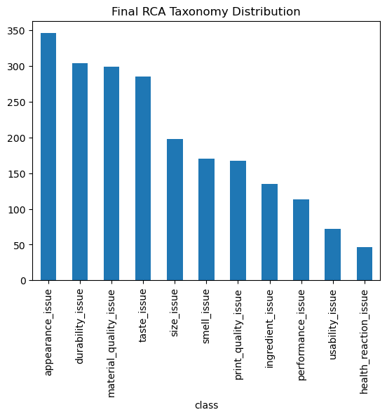
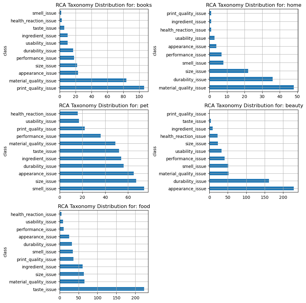
tag_frequency['class'].value_counts().head(20).plot(kind='bar')
plt.title('Final RCA Taxonomy Distribution')
plt.show()
pareto_df
| class | count | share_pct | review_count | rating | cum_share_freq | confidence | impact | cum_share_imp | rating_impact | cum_share_rating | |
|---|---|---|---|---|---|---|---|---|---|---|---|
| 5 | performance_issue | 113 | 15.398230 | 18.920354 | 4.384071 | 0.944288 | 2.991742 | 46.067532 | 1.000000 | 1.842701 | 0.110548 |
| 10 | usability_issue | 72 | 20.452778 | 17.152778 | 4.377778 | 0.977996 | 2.898824 | 59.288995 | 0.883839 | 1.803712 | 0.218758 |
| 2 | health_reaction_issue | 47 | 33.753191 | 13.723404 | 4.351064 | 1.000000 | 2.689438 | 90.777128 | 0.409953 | 1.745274 | 0.323461 |
| 8 | smell_issue | 170 | 32.791765 | 13.517647 | 4.377647 | 0.750000 | 2.675365 | 87.729938 | 0.509067 | 1.665021 | 0.423350 |
| 1 | durability_issue | 304 | 46.348355 | 22.233553 | 4.491447 | 0.304307 | 3.145597 | 145.793269 | 0.164711 | 1.599702 | 0.519321 |
| 9 | taste_issue | 285 | 26.456140 | 11.726316 | 4.390526 | 0.577715 | 2.543672 | 67.295742 | 0.749579 | 1.550301 | 0.612327 |
| 0 | appearance_issue | 346 | 40.557803 | 21.511561 | 4.547399 | 0.161985 | 3.114029 | 126.298176 | 0.307397 | 1.409413 | 0.696882 |
| 7 | size_issue | 198 | 19.982828 | 16.116162 | 4.530303 | 0.670412 | 2.840023 | 56.751695 | 0.947955 | 1.333950 | 0.776909 |
| 4 | material_quality_issue | 299 | 24.851839 | 15.732441 | 4.535117 | 0.444288 | 2.817349 | 70.016316 | 0.673552 | 1.309738 | 0.855484 |
| 3 | ingredient_issue | 135 | 31.724444 | 9.829630 | 4.475556 | 0.891386 | 2.382286 | 75.576695 | 0.594450 | 1.249377 | 0.930437 |
| 6 | print_quality_issue | 167 | 22.357485 | 13.347305 | 4.564671 | 0.828184 | 2.663562 | 59.550551 | 0.816857 | 1.159527 | 1.000000 |
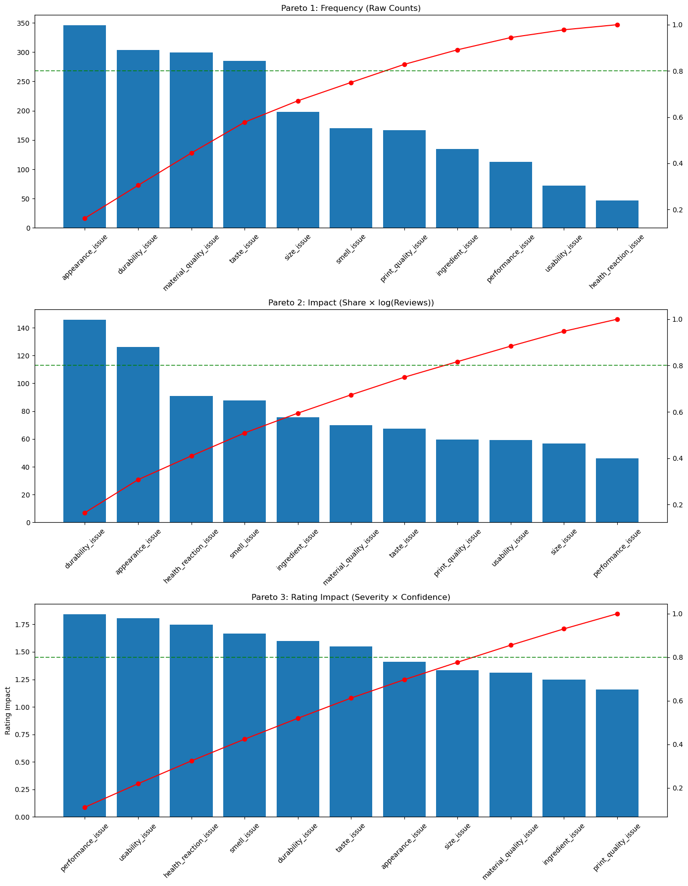
Pareto plots shows different perspectives on issue prioritization depending on the metric used. Based on frequency (Pareto 1) the most common issue classes are appearance_issue, durability_issue, material_quality_issue and taste_issue, which together account for a large proportion of all detected problems.
However when incorporating review volume through the impact score (Pareto 2)(share percentage weighted by review count confidence), durability_issue becomes the most important class, followed by appearance_issue, indicating that these issues are both widespread, due to stronger statistical support from review counts.
The rating impact (Pareto 3) analysis provides a different view by highlighting issues associated with lower customer satisfaction. Here performance_issue, usability_issue, and health_reaction_issue rank highest, suggesting that although these issues may not be the most frequent, they have a stronger negative effect on product ratings. In contrast, highly frequent issues such as appearance_issue and durability_issue show a lower rating impact, indicating that customers may tolerate them more than issues directly affecting product experience.
From a business perspective, frequency based metrics might help identify the largest sources of complaints, while rating impact highlights the issues most damaging to customer satisfaction. So an effective RCA prioritization strategy should consider both dimensions rather than relying solely on complaint volume.
Weighted Business Impact Score#
Root Cause Prioritization using a Weighted Business Impact Score
The proposed ranking approach is inspired by the Failure Mode and Effects Analysis (FMEA) methodology and uses a weighted business impact score to prioritize root causes.
def business_impact_score(share_pct: float, rating: float, review_count: int) -> float:
    # share_pct - how common, rating - how painfull, review_count - adds sconfidence/stability
    return (share_pct/100) * (5 - rating) * np.log1p(review_count)
rca_severity_weight = {
    'health_reaction_issue': 1.8,
    'durability_issue': 1.5,
    'performance_issue': 1.4,
    'ingredient_issue': 1.3,
    'material_quality_issue': 1.2,
    'taste_issue': 1.1,
    'smell_issue': 1.1,
    'size_issue': 1.0,
    'appearance_issue': 0.9,
    'print_quality_issue': 0.9,
    'usability_issue': 1.0,
}

def business_impact_score(
    frequency: int,
    review_count: int,
    rating: float,
    issue_class: str,
    prior_rate: float = 0.15,
    smoothing: int = 10,
) -> tuple[float]:
    issue_rate = (frequency + smoothing * prior_rate) / (review_count + smoothing) #avoids over ranking 1/2 or 2/2 cases
    rating_severity = max(0.15, (5 - rating) / 4) #small floor so rating 5 does not erase issues
    confidence = np.log1p(review_count) #more reviews is more confidence
    class_weight = rca_severity_weight.get(issue_class, 1.0)

    return (issue_rate, rating_severity, issue_rate * rating_severity * confidence * class_weight)
tag_frequency[['issue_rate', 'rating_severity', 'impact_score']] = tag_frequency.apply(
    lambda row: business_impact_score(
        row['frequency'], row['review_count'], row['rating'], row['class'],
    ), axis=1, result_type='expand'
)
tag_frequency.style.background_gradient(subset=['impact_score'], cmap='coolwarm')
tag_frequency[tag_frequency['category']=='books'].sort_values('impact_score', ascending=False).head(10)
| product_id | name | category | rating | price_kzt | tag_lemma | frequency | review_count | share_pct | class | issue_rate | rating_severity | impact_score | |
|---|---|---|---|---|---|---|---|---|---|---|---|---|---|
| 1550 | 2779736 | Разрушительная любовь | books | 4.6 | 4404.0 | клише | 29 | 30 | 96.7 | print_quality_issue | 0.762500 | 0.150 | 0.353486 |
| 67 | 389876 | Гарри Поттер и Философский камень | books | 4.3 | 7283.0 | перевод | 22 | 30 | 73.3 | print_quality_issue | 0.587500 | 0.175 | 0.317751 |
| 215 | 937477 | Богатый папа, бедный папа | books | 4.4 | 5816.0 | расклеиваться | 14 | 30 | 46.7 | durability_issue | 0.387500 | 0.150 | 0.299401 |
| 82 | 473259 | Кошки и котята | books | 4.9 | 2050.0 | порода | 10 | 23 | 43.5 | ingredient_issue | 0.348485 | 0.150 | 0.215963 |
| 206 | 875533 | Сказки барда Бидля | books | 4.8 | 6250.0 | перевод | 12 | 22 | 54.5 | print_quality_issue | 0.421875 | 0.150 | 0.178576 |
| 1553 | 2784038 | Кругом одни идиоты. 4 типа личности. Как найти... | books | 4.7 | 2094.0 | переплёт | 5 | 11 | 45.5 | durability_issue | 0.309524 | 0.150 | 0.173056 |
| 129 | 632472 | Бухгалтерский учет от азов до баланса. Практич... | books | 4.5 | 8226.0 | опечатка | 13 | 30 | 43.3 | print_quality_issue | 0.362500 | 0.150 | 0.168051 |
| 662 | 1493660 | Исследование о природе и причинах богатства на... | books | 4.7 | 3208.0 | переплёт | 4 | 8 | 50.0 | durability_issue | 0.305556 | 0.150 | 0.151059 |
| 378 | 1256282 | Дневник жены юмориста | books | 4.5 | 1047.0 | простой | 10 | 23 | 43.5 | print_quality_issue | 0.348485 | 0.150 | 0.149513 |
| 59 | 322768 | Золотое универсальное Таро. 78 карт | books | 4.6 | 13434.0 | позолота стираться | 5 | 21 | 23.8 | durability_issue | 0.209677 | 0.150 | 0.145827 |
tag_frequency.style.background_gradient(subset=['impact_score'], cmap='coolwarm')
tag_frequency[tag_frequency['category']=='home'].sort_values('impact_score', ascending=False).head(10)
| product_id | name | category | rating | price_kzt | tag_lemma | frequency | review_count | share_pct | class | issue_rate | rating_severity | impact_score | |
|---|---|---|---|---|---|---|---|---|---|---|---|---|---|
| 699 | 1607513 | ДМ Текстиль Полотенце махровое | home | 4.5 | 5522.0 | тонкий | 23 | 30 | 76.7 | material_quality_issue | 0.612500 | 0.15 | 0.378597 |
| 703 | 1607524 | ДМ Текстиль Полотенце махровое | home | 4.5 | 3361.0 | тонкий | 22 | 29 | 75.9 | material_quality_issue | 0.602564 | 0.15 | 0.368899 |
| 857 | 1766569 | ДМ Текстиль Полотенце махровое | home | 4.5 | 4378.0 | тонкий | 22 | 30 | 73.3 | material_quality_issue | 0.587500 | 0.15 | 0.363144 |
| 696 | 1607508 | ДМ Текстиль Полотенце махровое | home | 4.5 | 1790.0 | тонкий | 21 | 28 | 75.0 | material_quality_issue | 0.592105 | 0.15 | 0.358883 |
| 705 | 1607534 | ДМ Текстиль Полотенце махровое | home | 4.5 | 1579.0 | тонкий | 21 | 28 | 75.0 | material_quality_issue | 0.592105 | 0.15 | 0.358883 |
| 704 | 1607528 | ДМ Текстиль Полотенце махровое | home | 4.5 | 1579.0 | тонкий | 21 | 29 | 72.4 | material_quality_issue | 0.576923 | 0.15 | 0.353201 |
| 700 | 1607514 | ДМ Текстиль Полотенце махровое | home | 4.5 | 1579.0 | тонкий | 21 | 29 | 72.4 | material_quality_issue | 0.576923 | 0.15 | 0.353201 |
| 697 | 1607510 | ДМ Текстиль Полотенце махровое | home | 4.5 | 4352.0 | тонкий | 20 | 27 | 74.1 | material_quality_issue | 0.581081 | 0.15 | 0.348531 |
| 702 | 1607519 | ДМ Текстиль Полотенце махровое | home | 4.5 | 2419.0 | тонкий | 20 | 27 | 74.1 | material_quality_issue | 0.581081 | 0.15 | 0.348531 |
| 698 | 1607511 | ДМ Текстиль Полотенце махровое | home | 4.5 | 5142.0 | тонкий | 20 | 27 | 74.1 | material_quality_issue | 0.581081 | 0.15 | 0.348531 |
tag_frequency.style.background_gradient(subset=['impact_score'], cmap='coolwarm')
tag_frequency[tag_frequency['category']=='pet'].sort_values('impact_score', ascending=False).head(10)
| product_id | name | category | rating | price_kzt | tag_lemma | frequency | review_count | share_pct | class | issue_rate | rating_severity | impact_score | |
|---|---|---|---|---|---|---|---|---|---|---|---|---|---|
| 775 | 1660192 | Bonsy БИОошейник антипаразитарный для котят и ... | pet | 4.1 | 1026.0 | сильный запах | 20 | 24 | 83.3 | smell_issue | 0.632353 | 0.225 | 0.503778 |
| 777 | 1660198 | Bonsy БИОошейник антипаразитарный для котят и ... | pet | 4.1 | 1026.0 | сильный запах | 19 | 26 | 73.1 | smell_issue | 0.569444 | 0.225 | 0.464507 |
| 145 | 729892 | Пижон Мышь из натурального меха малая, 9×4×4 с... | pet | 3.7 | 810.0 | маленький | 13 | 28 | 46.4 | size_issue | 0.381579 | 0.325 | 0.417589 |
| 776 | 1660194 | Bonsy БИОошейник антипаразитарный для котят и ... | pet | 4.1 | 1026.0 | сильный запах | 15 | 23 | 65.2 | smell_issue | 0.500000 | 0.225 | 0.393284 |
| 1334 | 2433589 | Сибирская Кошка Наполнитель для кошачьего туал... | pet | 3.3 | 3633.0 | не_впитывать запах | 6 | 15 | 40.0 | smell_issue | 0.300000 | 0.425 | 0.388856 |
| 890 | 1810478 | Сибирская Кошка Наполнитель для кошачьего туал... | pet | 3.3 | 1725.0 | не_впитывать запах | 6 | 15 | 40.0 | smell_issue | 0.300000 | 0.425 | 0.388856 |
| 1600 | 2914453 | Сибирская Кошка Наполнитель для кошачьего туал... | pet | 3.3 | 6131.0 | не_впитывать запах | 6 | 15 | 40.0 | smell_issue | 0.300000 | 0.425 | 0.388856 |
| 508 | 1406213 | Mr.Fresh Expert Спрей «Защита от царапания» дл... | pet | 3.3 | 3274.0 | резкий запах | 5 | 8 | 62.5 | smell_issue | 0.361111 | 0.425 | 0.370934 |
| 99 | 554894 | Пижон Колтунорез боковой 9 лезвий | pet | 1.5 | 3511.0 | боль животный | 1 | 2 | 50.0 | health_reaction_issue | 0.208333 | 0.875 | 0.360482 |
| 257 | 1105450 | Monge Ветеринарный паштет для кошек при струви... | pet | 1.0 | 741.0 | запах | 2 | 2 | 100.0 | smell_issue | 0.291667 | 1.000 | 0.352471 |
tag_frequency.style.background_gradient(subset=['impact_score'], cmap='coolwarm')
tag_frequency[tag_frequency['category']=='beauty'].sort_values('impact_score', ascending=False).head(10)
| product_id | name | category | rating | price_kzt | tag_lemma | frequency | review_count | share_pct | class | issue_rate | rating_severity | impact_score | |
|---|---|---|---|---|---|---|---|---|---|---|---|---|---|
| 393 | 1290127 | Organic Kitchen Маска-лифтинг для лица «Укол к... | beauty | 4.6 | 1281.0 | жжение | 27 | 30 | 90.0 | health_reaction_issue | 0.712500 | 0.15 | 0.660613 |
| 253 | 1101085 | Art-Visage Тушь для ресниц суперобъемная «Chic... | beauty | 4.6 | 2887.0 | осыпаться | 29 | 30 | 96.7 | durability_issue | 0.762500 | 0.15 | 0.589143 |
| 222 | 989112 | Vivienne Sabo Тушь для ресниц с эффектом сцени... | beauty | 4.6 | 2530.0 | осыпаться | 29 | 30 | 96.7 | durability_issue | 0.762500 | 0.15 | 0.589143 |
| 1182 | 2279197 | Golden Rose Лак для ногтей «Keratin nail color... | beauty | 4.6 | 882.0 | полосит | 28 | 30 | 93.3 | durability_issue | 0.737500 | 0.15 | 0.569827 |
| 1174 | 2279097 | Golden Rose Лак для ногтей «Keratin nail color... | beauty | 4.6 | 882.0 | полосит | 28 | 30 | 93.3 | durability_issue | 0.737500 | 0.15 | 0.569827 |
| 1241 | 2325414 | Golden Rose Лак для ногтей «Keratin nail color... | beauty | 4.6 | 882.0 | полосит | 28 | 30 | 93.3 | durability_issue | 0.737500 | 0.15 | 0.569827 |
| 1175 | 2279143 | Golden Rose Лак для ногтей «Keratin nail color... | beauty | 4.6 | 882.0 | полосит | 28 | 30 | 93.3 | durability_issue | 0.737500 | 0.15 | 0.569827 |
| 1187 | 2279209 | Golden Rose Лак для ногтей «Keratin nail color... | beauty | 4.6 | 882.0 | полосит | 27 | 29 | 93.1 | durability_issue | 0.730769 | 0.15 | 0.559235 |
| 1207 | 2279260 | Golden Rose Лак для ногтей «Keratin nail color... | beauty | 4.6 | 882.0 | полосит | 27 | 29 | 93.1 | durability_issue | 0.730769 | 0.15 | 0.559235 |
| 1192 | 2279221 | Golden Rose Лак для ногтей «Keratin nail color... | beauty | 4.6 | 882.0 | полосит | 27 | 29 | 93.1 | durability_issue | 0.730769 | 0.15 | 0.559235 |
tag_frequency[tag_frequency['category']=='food'].sort_values('impact_score', ascending=False).head(10)
| product_id | name | category | rating | price_kzt | tag_lemma | frequency | review_count | share_pct | class | issue_rate | rating_severity | impact_score | |
|---|---|---|---|---|---|---|---|---|---|---|---|---|---|
| 954 | 1879352 | Иван да Марья Рожки нутовые без глютена | food | 4.2 | 1716.0 | развариваться | 10 | 12 | 83.3 | durability_issue | 0.522727 | 0.200 | 0.402231 |
| 953 | 1879322 | Иван да Марья Рожки гороховые без глютена | food | 4.2 | 1439.0 | развариваться | 10 | 12 | 83.3 | durability_issue | 0.522727 | 0.200 | 0.402231 |
| 1308 | 2409789 | Корона Чернослив | food | 4.1 | 778.0 | плесень | 9 | 15 | 60.0 | ingredient_issue | 0.420000 | 0.225 | 0.340613 |
| 1907 | 3893080 | Вкусы мира Конфеты «Манго-шарики в какао-глазури» | food | 4.1 | 590.0 | глазурь | 5 | 12 | 41.7 | health_reaction_issue | 0.295455 | 0.225 | 0.306920 |
| 902 | 1832160 | Bestofindia Чай черный «Масала» | food | 4.0 | 1487.0 | гранулированный | 7 | 15 | 46.7 | ingredient_issue | 0.340000 | 0.250 | 0.306371 |
| 1695 | 3119759 | Makfa Макароны «Королевские ракушки» | food | 4.5 | 545.0 | развариваться | 10 | 12 | 83.3 | durability_issue | 0.522727 | 0.150 | 0.301673 |
| 870 | 1788782 | Трапеза Пудра сахарная нетающая шоколадная | food | 4.4 | 2158.0 | таять | 15 | 23 | 65.2 | material_quality_issue | 0.500000 | 0.150 | 0.286025 |
| 1569 | 2846656 | Foco Кокосовое молоко органическое | food | 4.6 | 1049.0 | расслоение | 12 | 28 | 42.9 | durability_issue | 0.355263 | 0.150 | 0.269162 |
| 1226 | 2285577 | TopLife Псиллиум | food | 4.5 | 4172.0 | комковаться | 11 | 23 | 47.8 | performance_issue | 0.378788 | 0.150 | 0.252800 |
| 903 | 1832160 | Bestofindia Чай черный «Масала» | food | 4.0 | 1487.0 | мало специя | 5 | 15 | 33.3 | ingredient_issue | 0.260000 | 0.250 | 0.234284 |
tag_frequency.to_csv('data/tag_ferquency_ranked.csv', index=False)